Posts in HOW To’s

Autoscaling an Instance Group with Custom Cloud Monitoring Metrics

Overview

Here, we will create a Compute Engine managed instance group that autoscale based on the value of a custom Cloud Monitoring metric.

What you’ll learn

  • Deploy an autoscaling Compute Engine instance group.
  • Create a custom metric used to scale the instance group.
  • Use the Cloud Console to visualize the custom metric and instance group size.

Application Architecture

The autoscaling application uses a Node.js script installed on Compute Engine instances. The script reports a numeric value to a Cloud monitoring metric. You do not need to know Node.js or JavaScript for this lab. In response to the value of the metric, the application autoscale the Compute Engine instance group up or down as needed.

The Node.js script is used to seed a custom metric with values that the instance group can respond to. In a production environment, you would base autoscaling on a metric that is relevant to your use case.

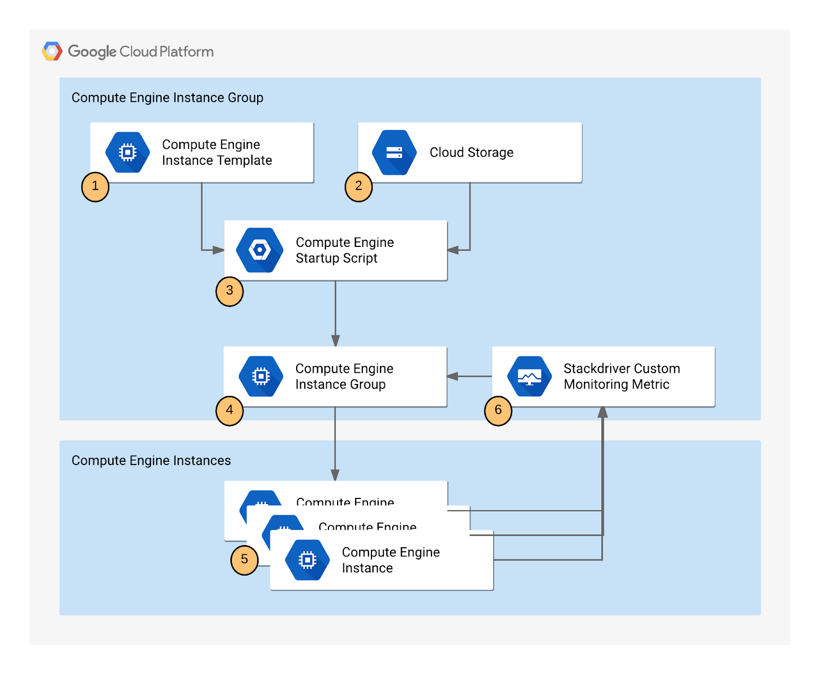
The application includes the following components:

  1. Compute Engine instance template – A template used to create each instance in the instance group.
  2. Cloud Storage – A bucket used to host the startup script and other script files.
  3. Compute Engine startup script – A startup script that installs the necessary code components on each instance. The startup script is installed and started automatically when an instance starts. When the startup script runs, it in turn installs and starts code on the instance that writes values to the Cloud monitoring custom metric.
  4. Compute Engine instance group – An instance group that autoscale based on the Cloud monitoring metric values.
  5. Compute Engine instances – A variable number of Compute Engine instances.
  6. Custom Cloud Monitoring metric – A custom monitoring metric used as the input value for Compute Engine instance group autoscaling.
Lab architecture diagram

Task 1. Creating the application

Creating the autoscaling application requires downloading the necessary code components, creating a managed instance group, and configuring autoscaling for the managed instance group.

Uploading the script files to Cloud Storage

During autoscaling, the instance group will need to create new Compute Engine instances. When it does, it creates the instances based on an instance template. Each instance needs a startup script. Therefore, the template needs a way to reference the startup script. Compute Engine supports using Cloud Storage buckets as a source for your startup script. In this section, you will make a copy of the startup script and application files for a sample application used by this lab that pushes a pattern of data into a custom Cloud logging metric that you can then use to configure as the metric that controls the autoscaling behavior for an autoscaling group.

Note: There is a pre-existing instance template and group that has been created automatically by the lab that is already running. Autoscaling requires at least 30 minutes to demonstrate both scale-up and scale-down behavior, and you will examine this group later to see how scaling is controlled by the variations in the custom metric values generated by the custom metric scripts.

Task 2. Create a bucket

  1. In the Cloud Console, scroll down to Cloud Storage from the Navigation menu, then click Create.
  2. Give your bucket a unique name, but don’t use a name you might want to use in another project. For details about how to name a bucket, see the bucket naming guidelines. This bucket will be referenced as YOUR_BUCKET throughout the lab.
  3. Accept the default values then click Create.

Click Confirm for Public access will be prevented pop-up if prompted.

When the bucket is created, the Bucket details page opens.

  1. Next, run the following command in Cloud Shell to copy the startup script files from the lab default Cloud Storage bucket to your Cloud Storage bucket. Remember to replace <YOUR BUCKET> with the name of the bucket you just made:

gsutil cp -r gs://spls/gsp087/* gs://<YOUR BUCKET>

  1. After you upload the scripts, click Refresh on the Bucket details page. Your bucket should list the added files.

Understanding the code components

  • Startup.sh – A shell script that installs the necessary components to each Compute Engine instance as the instance is added to the managed instance group.
  • writeToCustomMetric.js – A Node.js snippet that creates a custom monitoring metric whose value triggers scaling. To emulate real-world metric values, this script varies the value over time. In a production deployment, you replace this script with custom code that reports the monitoring metric that you’re interested in, such as a processing queue value.
  • Config.json – A Node.js config file that specifies the values for the custom monitoring metric and is used in writeToCustomMetric.js.
  • Package.json – A Node.js package file that specifies standard installation and dependencies for writeToCustomMetric.js.
  • writeToCustomMetric.sh – A shell script that continuously runs the writeToCustomMetric.js program on each Compute Engine instance.

Task 3. Creating an instance template

Now create a template for the instances that are created in the instance group that will use autoscaling. As part of the template, you specify the location (in Cloud Storage) of the startup script that should run when the instance starts.

  1. In the Cloud Console, click Navigation menu > Compute Engine > Instance templates.
  2. Click Create Instance Template at the top of the page.
  3. Name the instance template autoscaling-instance01.
  4. Scroll down, click Advanced options.
  5. In the Metadata section of the Management tab, enter these metadata keys and values, clicking the + Add item button to add each one. Remember to substitute your bucket name for the [YOUR_BUCKET_NAME] placeholder:
KeyValue
startup-script-urlgs://[YOUR_BUCKET_NAME]/startup.sh
gcs-bucketgs://[YOUR_BUCKET_NAME]
  1. Click Create.

Task 4. Creating the instance group

  1. In the left pane, click Instance groups.
  2. Click Create instance group at the top of the page.
  3. Name: autoscaling-instance-group-1.
  4. For Instance template, select the instance template you just created.
  5. Set Autoscaling mode to Off: do not autoscale.

You’ll edit the autoscaling setting after the instance group has been created. Leave the other settings at their default values.

  1. Click Create.

Note: You can ignore the Autoscaling is turned off. The number of instances in the group won't change automatically. The autoscaling configuration is preserved. warning next to your instance group.

Task 5. Verifying that the instance group has been created

Wait to see the green check mark next to the new instance group you just created. It might take the startup script several minutes to complete installation and begin reporting values. Click Refresh if it seems to be taking more than a few minutes.

Note: If you see a red icon next to the other instance group that was pre-created by the lab, you can ignore this warning. The instance group reports a warning for up to ten minutes as it is initializing. This is expected behavior.

Task 6. Verifying that the Node.js script is running

The custom metric custom.googleapis.com/appdemo_queue_depth_01 isn’t created until the first instance in the group is created and that instance begins reporting custom metric values.

You can verify that the writeToCustomMetric.js script is running on the first instance in the instance group by checking whether the instance is logging custom metric values.

  1. Still in the Compute Engine Instance groups window, click the name of the autoscaling-instance-group-1 to display the instances that are running in the group.
  2. Scroll down and click the instance name. Because autoscaling has not started additional instances, there is just a single instance running.
  3. In the Details tab, in the Logs section, click Cloud Logging link to view the logs for the VM instance.
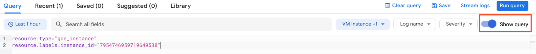
  4. Wait a minute or 2 to let some data accumulate. Enable the Show query toggle, you will see resource.type and resource.labels.instance_id in the Query preview box.
 Query preview box
  1. Add “nodeapp” as line 3, so the code looks similar to this:
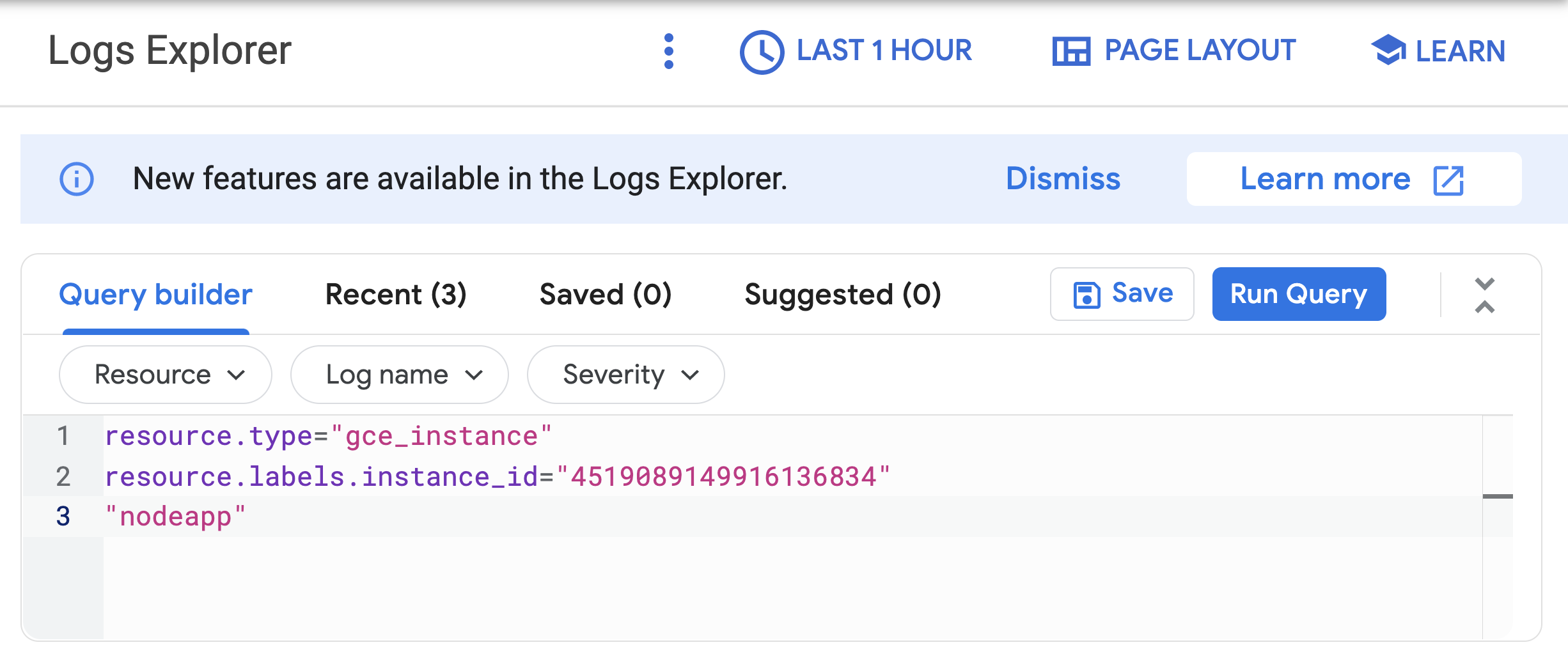
Line 1: resource.type="gce.instance". Line 2: resource.labels.instance_id="4519089149916136834". Line 3: "nodeapp"
  1. Click Run query.

If the Node.js script is being executed on the Compute Engine instance, a request is sent to the API, and log entries that say Finished writing time series data appear in the logs.

Note: If you don’t see this log entry, the Node.js script isn’t reporting the custom metric values. Check that the metadata was entered correctly. If the metadata is incorrect, it might be easiest to restart the lab.

Task 7. Configure autoscaling for the instance group

After you’ve verified that the custom metric is successfully reporting data from the first instance, the instance group can be configured to autoscale based on the value of the custom metric.

  1. In the Cloud Console, go to Compute Engine > Instance groups.
  2. Click the autoscaling-instance-group-1 group.
  3. Under Autoscaling click Configure.
  4. Set Autoscaling mode to On: add and remove instances to the group.
  5. Set Minimum number of instances1 and Maximum number of instances3
  6. Under Autoscaling signals click ADD SIGNAL to edit metric. Set the following fields, leave all others at the default value.
  • Signal typeCloud Monitoring metric new. Click Configure.
  • Under Resource and metric click SELECT A METRIC and navigate to VM Instance > Custom metrics > Custom/appdemo_queue_depth_01.
  • Click Apply.
  • Utilization target150When custom monitoring metric values are higher or lower than the Target value, the autoscaler scales the managed instance group, increasing or decreasing the number of instances. The target value can be any double value, but for this lab, the value 150 was chosen because it matches the values being reported by the custom monitoring metric.
  • Utilization target typeGauge. Click Select.The Gauge setting specifies that the autoscaler should compute the average value of the data collected over the last few minutes and compare it to the target value. (By contrast, setting Target mode to DELTA_PER_MINUTE or DELTA_PER_SECOND autoscales based on the observed rate of change rather than an average value.)
  1. Click Save.

Task 8. Watching the instance group perform autoscaling

The Node.js script varies the custom metric values it reports from each instance over time. As the value of the metric goes up, the instance group scales up by adding Compute Engine instances. If the value goes down, the instance group detects this and scales down by removing instances. As noted earlier, the script emulates a real-world metric whose value might similarly fluctuate up and down.

Next, you will see how the instance group is scaling in response to the metric by clicking the Monitoring tab to view the Autoscaled size graph.

  1. In the left pane, click Instance groups.
  2. Click the builtin-igm instance group in the list.
  3. Click the Monitoring tab.
  4. Enable Auto Refresh.

Since this group had a head start, you can see the autoscaling details about the instance group in the autoscaling graph. The autoscaler will take about five minutes to correctly recognize the custom metric and it can take up to ten minutes for the script to generate sufficient data to trigger the autoscaling behavior.

Monitoring tabbed page displaying two monitoring graphs

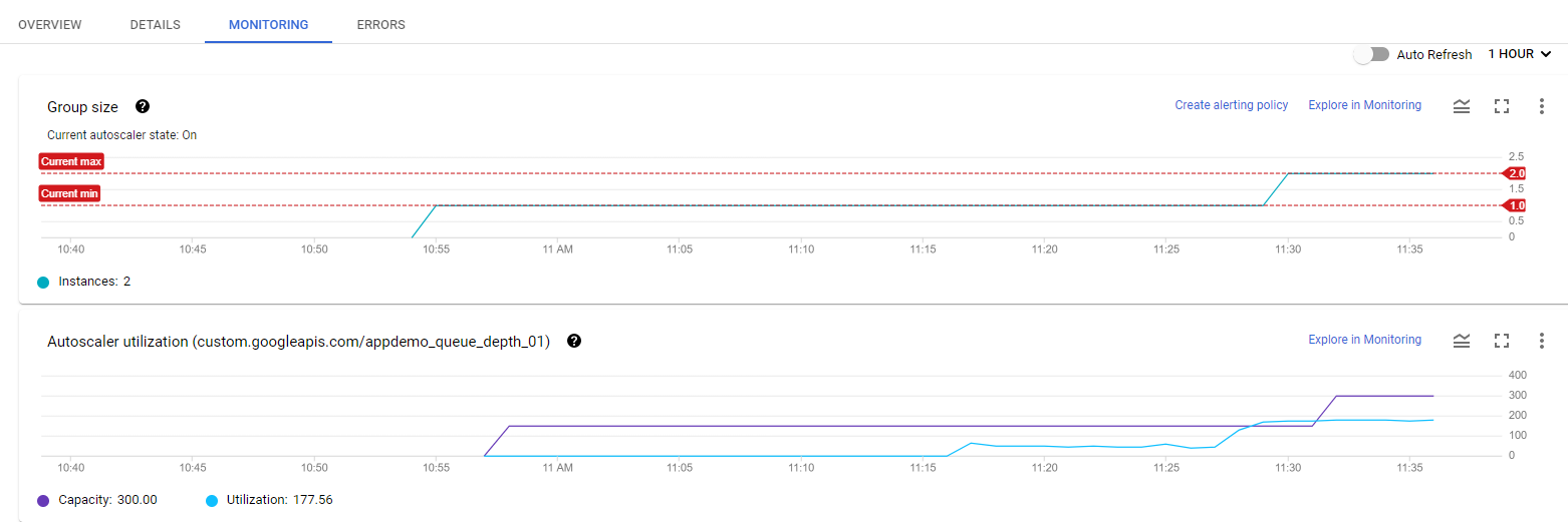
Hover your mouse over the graphs to see more details.

You can switch back to the instance group that you created to see how it’s doing (there may not be enough time left in the lab to see any autoscaling on your instance group).

For the remainder of the time in your lab, you can watch the autoscaling graph move up and down as instances are added and removed.

Task 9. Autoscaling example

Read this autoscaling example to see how the capacity and number of autoscaled instances can work in a larger environment.

The number of instances depicted in the top graph changes as a result of the varying aggregate levels of the custom metric property values reported in the lower graph. There is a slight delay of up to five minutes after each instance starts up before that instance begins to report its custom metric values. While your autoscaling starts up, read through this graph to understand what will be happening:

Members tabbed page displaying a graph with several data points

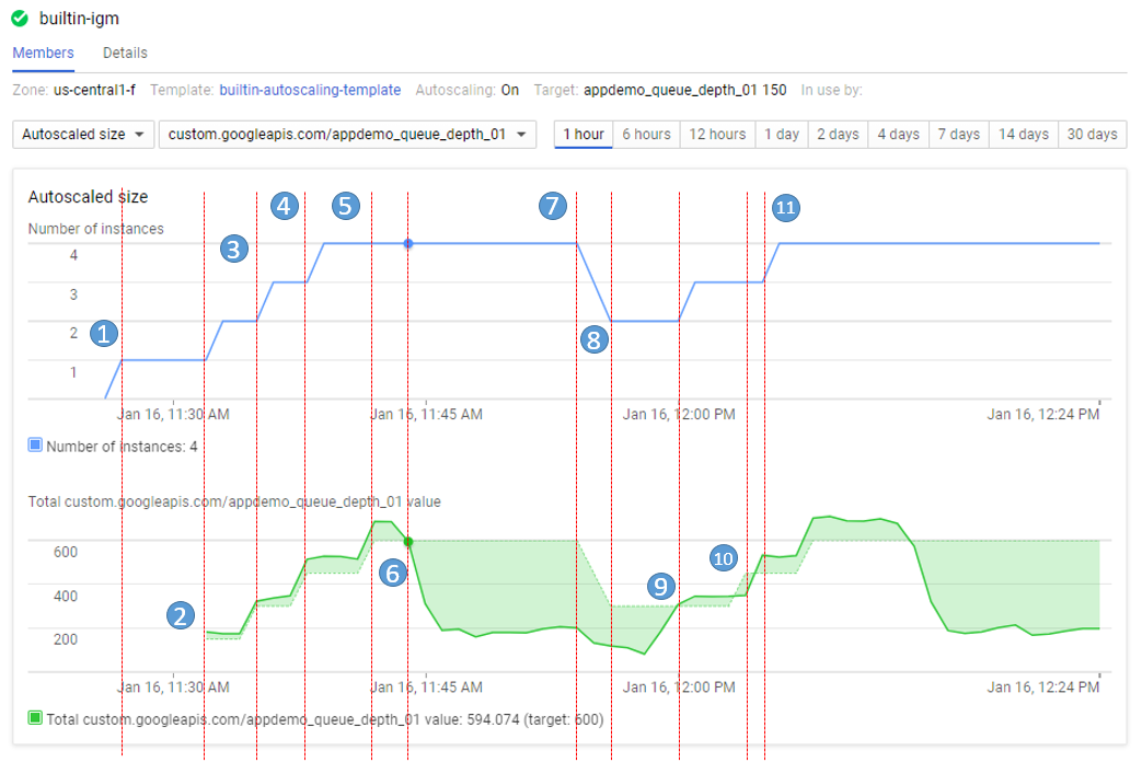
The script starts by generating high values for approximately 15 minutes in order to trigger scale-up behavior.

  • 11:27 Autoscaling Group starts with a single instance. The aggregate custom metric target is 150.
  • 11:31 Initial metric data acquired. As the metric is greater than the target of 150 the autoscaling group starts a second instance.
  • 11:33 Custom metric data from the second instance starts to be acquired. The aggregate target is now 300. As the metric value is above 300 the autoscaling group starts the third instance.
  • 11:37 Custom metric data from the third instance starts to be acquired. The aggregate target is now 450. As the cumulative metric value is above 450 the autoscaling group starts the fourth instance.
  • 11:42 Custom metric data from the fourth instance starts to be acquired. The aggregate target is now 600. The cumulative metric value is now above the new target level of 600 but since the autoscaling group size limit has been reached no additional scale-up actions occur.
  • 11:44 The application script has moved into a low metric 15-minute period. Even though the cumulative metric value is below the target of 600 scale-down must wait for a ten-minute built-in scale-down delay to pass before making any changes.
  • 11:54 Custom metric data has now been below the aggregate target level of 600 for a four-node cluster for over 10 minutes. Scale-down now removes two instances in quick succession.
  • 11:56 Custom metric data from the removed nodes is eliminated from the autoscaling calculation and the aggregate target is reduced to 300.
  • 12:00 The application script has moved back into a high metric 15-minute period. The cumulative custom metric value has risen above the aggregate target level of 300 again so the autoscaling group starts a third instance.
  • 12:03 Custom metric data from the new instance have been acquired but the cumulative values reported remain below the target of 450 so autoscaling makes no changes.
  • 12:04 Cumulative custom metric values rise above the target of 450 so autoscaling starts the fourth instance.

Congratulations!

You have successfully created a managed instance group that autoscale based on the value of a custom metric.

Manually Migrate Data Between Redshift Clusters

You have been presented with a few pain points to solve around your company’s Redshift solution. The original Redshift cluster that was launched for the company’s analytics stack has become underpowered over time. Several groups wish to create incremental backups of certain tables to S3 in a format that can be plugged into data lake solutions, as well as other groups wishing to have select pieces of the main Redshift schema splintered to new department-specific clusters.

You’ve come up with a plan to utilize the UNLOAD and COPY commands to facilitate all of the above and need to test a proof of concept to ensure that all pain points above can be addressed in this manner.

Read More

Using Secrets Manager to Authenticate with an RDS Database Using Lambda

Introduction

AWS Secrets Manager helps you protect the secrets needed to access your applications, services, and IT resources. The service enables you to easily rotate, manage, and retrieve database credentials, API keys, and other secrets throughout their lifecycle. In this lab, we connect to a MySQL RDS database from an AWS Lambda function using a username and password, and then we hand over credential management to the AWS Secrets Manager service. We then use the Secrets Manager API to connect to the database instead of hard-coding credentials in our Lambda function. By the end of this lab, you will understand how to store a secret in AWS Secrets Manager and access it from a Lambda function.

Solution

Log in to the live AWS environment using the credentials provided. Use an incognito or private browser window to ensure you’re using the lab account rather than your own.

Make sure you’re in the N. Virginia (us-east-1) region throughout the lab.

Download the MySQL Library ZIP file you’ll need for the first lab objective.

Create Lambda Function

  1. Navigate to Lambda > Functions.
  2. Click Create function.
  3. Make sure the Author from scratch option at the top is selected, and then use the following settings:
    • Function name: Enter testRDS.
    • Runtime: Select Node.js 14.x.
  4. Expand Advanced settings, and set the following values:
    • Enable VPC: Check the box.
    • VPC: Select the lab-provided VPC.
    • Subnets: Enter Public and select the two subnets that have Public in their name/ID.
    • Security groups: Select the lab-provided Database-Security-Group security group (not the default security group).
  5. Click Create function.
    • It may take 5–10 minutes to finish creating.
  6. Click the Configuration tab.
  7. Click Edit.
  8. Under Timeout, change it to 6 seconds.
  9. Click Save.
  10. In the left-hand menu, click Layers.
  11. Click Create layer.
  12. Set the following values:
    • Name: Enter mysql.
    • Upload a .zip file: Click Upload and upload the MySQL Library ZIP file you downloaded earlier.
    • Compatible runtimesNode.js 14.x
  13. Click Create.
  14. Click Functions in the left-hand menu.
  15. Click your testRDS function.
  16. In the Function overview section, click Layers under testRDS.
  17. In the Layers section, click Add a layer.
  18. Select Custom layers, and set the following values:
    • Custom layers: Select mysql.
    • Version: Select 1.
  19. Click Add.

Copy Code into Lambda Function

  1. In the Code source section, expand testRDS > index.js.
  2. Select the existing code in the index.js tab and replace it with the following:var mysql = require('mysql'); exports.handler = (event, context, callback) => { var connection = mysql.createConnection({ host: "<RDS Endpoint>", user: "username", password: "password", database: "example", }); connection.query('show tables', function (error, results, fields) { if (error) { connection.destroy(); throw error; } else { // connected! console.log("Query result:"); console.log(results); callback(error, results); connection.end(function (err) { callback(err, results);}); } }); };
  3. In a new browser tab, navigate to RDS > DB Instances.
  4. Click the listed database.
  5. Copy the endpoint (in the Connectivity & security section) and paste it into a plaintext file (you’ll need it a couple times during the lab).
  6. Back in the Lambda function code, replace <RDS Endpoint> on line 6 with the endpoint you just copied.
  7. Click Deploy.
  8. Click Test.
  9. In the Configure test event dialog, enter an Event name of test.
  10. Click Save.
  11. Click Test again.
    • The Response should only be two square brackets, which is correct since we don’t have any tables defined in this database.
  12. Click the index.js tab.
  13. Replace line 12 with the following:connection.query('CREATE TABLE pet (name VARCHAR(20), species VARCHAR(20))',function (error, results, fields) {
  14. Click Deploy.
  15. Click Test.
    • This time, the Response should have information within curly brackets.
  16. Click the index.js tab.
  17. Undo the code change (Ctrl+Z or Cmd+Z) to get it back to the original code we pasted in.
  18. Click Deploy.
  19. Click Test.
    • This time, we should see the pet table listed in the Response.

Create a Secret in Secrets Manager

  1. In a new browser tab, navigate to Secrets Manager.
  2. Click Store a new secret.
  3. With Credentials for Amazon RDS database selected, set the following values:
    • User name: Enter username.
    • Password: Enter password.
    • Encryption key: Leave as the default.
    • Database: Select the listed DB instance.
  4. Click Next.
  5. On the next page, give it a Secret name of RDScredentials.
  6. Leave the rest of the defaults, and click Next.
  7. On the next page, set the following values:
    • Automatic rotation: Toggle to enable it.
    • Schedule expression builder: Select.
    • Time unit: Change it to Days1.
    • Create a rotation function: Select.
    • SecretsManager: Enter rotateRDS.
    • Use separate credentials to rotate this secret: Select No.
  8. Click Next.
  9. In the Sample code section, ensure the region is set to us-east-1.
  10. Click Store.
    • It may take 5–10 minutes to finish the configuration.
  11. Once it’s done, click RDScredentials.
  12. In the Secret value section, click Retrieve secret value.
    • You should see the password is now a long string rather than password.
    • If yours still says password, give it a few minutes and refresh the page. Your Lambda function may still be in the process of getting set up.
  13. Back in the Lambda function, click Test.
    • You will see errors saying access is denied because the password has changed.
  14. Click the index.js tab.
  15. Select all the code and replace it with the following:var mysql = require('mysql'); var AWS = require('aws-sdk'), region = "us-east-1", secretName = "RDScredentials", secret, decodedBinarySecret; var client = new AWS.SecretsManager({ region: "us-east-1" }); exports.handler = (event, context, callback) => { client.getSecretValue({SecretId: secretName}, function(err, data) { if (err) { console.log(err); } else { // Decrypts secret using the associated KMS CMK. // Depending on whether the secret is a string or binary, one of these fields will be populated. if ('SecretString' in data) { secret = data.SecretString; } else { let buff = new Buffer(data.SecretBinary, 'base64'); decodedBinarySecret = buff.toString('ascii'); } } var parse = JSON.parse(secret); var password = parse.password; var connection = mysql.createConnection({ host: "<RDS Endpoint>", user: "username", password: password, database: "example", }); connection.query('show tables', function (error, results, fields) { if (error) { connection.destroy(); throw error; } else { // connected! console.log("Query result:"); console.log(results); callback(error, results); connection.end(function (err) { callback(err, results);}); } }); }); };
  16. Replace <RDS Endpoint> with the value you copied earlier.
  17. Click Deploy.

Work with AWS VPC Flow Logs for Network Monitoring

Monitoring network traffic is a critical component of security best practices to meet compliance requirements, investigate security incidents, track key metrics, and configure automated notifications. AWS VPC Flow Logs captures information about the IP traffic going to and from network interfaces in your VPC. In this hands-on lab, we will set up and use VPC Flow Logs published to Amazon CloudWatch, create custom metrics and alerts based on the CloudWatch logs to understand trends and receive notifications for potential security issues, and use Amazon Athena to query and analyze VPC Flow Logs stored in S3.

Read More

Welcome Metricbeat from the beats family

Deploy Metricbeat on all your Linux, Windows, and Mac hosts, connect it to Elasticsearch and voila: you get system-level CPU usage, memory, file system, disk IO, and network IO statistics, as well as top-like statistics for every process running on your systems. Metricbeats is an open-source shipping agent used to collect and ship operating system and service metrics to one or more destinations, including Logstash.

Step 1 – Install Metricbeat

deb (Debian/Ubuntu/Mint)

sudo apt-get install apt-transport-https
wget -qO - https://artifacts.elastic.co/GPG-KEY-elasticsearch | sudo apt-key add -
echo 'deb https://artifacts.elastic.co/packages/oss-6.x/apt stable main' | sudo tee /etc/apt/sources.list.d/beats.list
sudo apt-get update && sudo apt-get install metricbeat

rpm (CentOS/RHEL/Fedora)

sudo rpm --import https://artifacts.elastic.co/GPG-KEY-elasticsearch
echo "[elastic-6.x]
name=Elastic repository for 6.x packages
baseurl=https://artifacts.elastic.co/packages/oss-6.x/yum
gpgcheck=1
gpgkey=https://artifacts.elastic.co/GPG-KEY-elasticsearch
enabled=1
autorefresh=1
type=rpm-md" | sudo tee /etc/yum.repos.d/elastic-beats.repo

sudo yum install metricbeat

macOS

curl -L -O https://artifacts.elastic.co/downloads/beats/metricbeat/metricbeat-oss-6.7.1-darwin-x86_64.tar.gz 
tar xzvf metricbeat-oss-6.7.1-darwin-x86_64.tar.gz

Windows

  • Download the Metricbeat Windows zip file from the official downloads page.
  • Extract the contents of the zip file into C:\Program Files.
  • Rename the metricbeat-<version>-windows directory to Metricbeat.
  • Open a PowerShell prompt as an Administrator (right-click the PowerShell icon and select Run As Administrator). If you are running Windows XP, you may need to download and install PowerShell.
  • Run the following commands to install Metricbeat as a Windows service:PS > cd 'C:\Program Files\Metricbeat' PS C:\Program Files\Metricbeat> .\install-service-metricbeat.ps1`   If script execution is disabled on your system, you need to set the execution policy for the current session to allow the script to run. For example: PowerShell.exe -ExecutionPolicy UnRestricted -File .\install-service-metricbeat.ps1

My OS isn’t here! Don’t see your system? Check out the official downloads page for more options (including 32-bit versions).

Step 2 – Locate the configuration file

deb/rpm : /etc/metricbeat/metricbeat.yml
mac/win :<EXTRACTED_ARCHIVE>/metricbeat.yml

Step 3 – Configure the Modules

Setup the data you wish to send us, by editing the modules. Examples of these settings are found in, in the same folder as the configuration file. The system status module is enabled by default to collect metrics about your servers, such as CPU usage, memory usage, network IO metrics, and process statistics:

metricbeat.modules:
- module: system
  metricsets:
    - cpu
    - filesystem
    - memory
    - network
    - process
  enabled: true
  period: 10s
  processes: ['.*']
  cpu_ticks: false

  There’s also a large range of modules to collect metrics see here.

Step 4 – Configure output

We’ll be shipping to Logstash so that we have the option to run filters before the data is indexed.
Comment out the elasticsearch output block.

## Comment out elasticsearch output
#output.elasticsearch:
#  hosts: ["localhost:9200"]

Uncomment and change the logstash output to match below.

output.logstash:
    hosts: ["your-logstash-host:your-port"]
    loadbalance: true
    ssl.enabled: true
Step 5 – Validate configuration

Let’s check the configuration file is syntactically correct.

deb/rpm

sudo metricbeat -e -c /etc/metricbeat/metricbeat.yml

macOS

cd <EXTRACTED_ARCHIVE>
./metricbeat -e -c metricbeat.yml

Windows

cd <EXTRACTED_ARCHIVE>
metricbeat.exe -e -c metricbeat.yml
Step 6 – Start metricbeat

Ok, time to start ingesting data!

deb/rpm

sudo systemctl enable metricbeat
sudo systemctl start metricbeat

mac

./metricbeat

Windows

Start-Service metricbeat

With this, you have installed & configured MetricBeat for your environment. Stay tuned for others from the Beats family and also the ElasticSearch Stack Installation.

vCSA 6.x Upgrade error: “No networks on the host. Cannot proceed with the installation.”

Recently during the vCSA 6.0 to 6.7 upgrade process, I encountered an error while deploying the new vCenter server appliance with an embedded PSC on the vCSA 6.7 installer.

The problem

In my case, I was trying to upgrade vCSA 6.0. If you notice that the network section is empty:

I cannot proceed, because of the error and it shows:

No networks on the host. Cannot proceed with the installation.

The Solution

The configuration on ESXi hosts and VCenter looked OK and obviously, it had port groups created in a standard virtual switch.

So the issue was that I didn’t have “VM Network” port group that is a default port group that is created once you deploy an ESXi host. In my case, it was auto-deployed with different port groups and that one didn’t exist.

Hence, as soon as I created a port group called “VM Network” in the host that I am trying to deploy the vCSA, it worked!

Now, I can see the port group and I was able to continue the installation with success!

I hope this worked for you as well.

GCP Series-Getting Started with BigQuery

Overview

In this lab, you load a web server log into a BigQuery table. After loading the data, you query it using the BigQuery web user interface and the BigQuery CLI.

BigQuery helps you perform interactive analysis of petabyte-scale databases, and it enables near-real time analysis of massive datasets. It offers a familiar SQL 2011 query language and functions.

Data stored in BigQuery is highly durable. Google stores your data in a replicated manner by default and at no additional charge for replicas. With BigQuery, you pay only for the resources you use. Data storage in BigQuery is inexpensive. Queries incur charges based on the amount of data they process: when you submit a query, you pay for the compute nodes only for the duration of that query. You don’t have to pay to keep a compute cluster up and running.

Using BigQuery involves interacting with a number of Google Cloud Platform resources, including projects (covered elsewhere in this course), datasets, tables, and jobs. This lab introduces you to some of these resources, and this brief introduction summarizes their role in interacting with BigQuery.

Datasets: A dataset is a grouping mechanism that holds zero or more tables. A dataset is the lowest level unit of access control. Datasets are owned by GCP projects. Each dataset can be shared with individual users.

Tables: A table is a row-column structure that contains actual data. Each table has a schema that describes strongly typed columns of values. Each table belongs to a dataset.

Objectives

  • Load data from Cloud Storage into BigQuery.
  • Perform a query on the data in BigQuery.

Task 1: Load data from Cloud Storage into BigQuery

  1. In the Console, on the Navigation menu () click BigQuery then click Done.
  2. Create a new dataset within your project by selecting your project in the Resources section, then clicking on CREATE DATASET on the right.
  3. In the Create Dataset dialog, for Dataset ID, type logdata.
  4. For Data location, select the continent closest to the region. click Create dataset.
  5. Create a new table in the logdata to store the data from the CSV file.
  6. Click on Create Table. On the Create Table page, in the Source section:
  • For Create table from, choose select Google Cloud Storage, and in the field, typegs://cloud-training/gcpfci/access_log.csv.
  • Verify File format is set to CSV.

Note: When you have created a table previously, the Create from Previous Job option allows you to quickly use your settings to create similar tables.

  1. In the Destination section:
  • For Dataset name, leave logdata selected.
  • For Table name, type accesslog.
  • For Table typeNative table should be selected and unchangeable.
  1. Under Schema section, for Auto detect check the Schema and input Parameters.
  2. Accept the remaining default values and click Create Table.BigQuery creates a load job to create the table and upload data into the table (this may take a few seconds).
  3. (Optional) To track job progress, click Job History.
  4. When the load job is complete, click logdata > accesslog.
  5. On the Table Details page, click Details to view the table properties, and then click Preview to view the table data.Each row in this table logs a hit on a web server. The first field, string_field_0, is the IP address of the client. The fourth through ninth fields log the day, month, year, hour, minute, and second at which the hit occurred. In this activity, you will learn about the daily pattern of load on this web server.

Task 2: Perform a query on the data using the BigQuery web UI

In this section of the lab, you use the BigQuery web UI to query the accesslog table you created previously.

  1. In the Query editor window, type (or copy-and-paste) the following query:
  2. Because you told BigQuery to automatically discover the schema when you load the data, the hour of the day during which each web hit arrived is in a field called int_field_6.select int64_field_6 as hour, count(*) as hitcount from logdata.accesslog group by hour order by hourNotice that the Query Validator tells you that the query syntax is valid (indicated by the green check mark) and indicates how much data the query will process. The amount of data processed allows you to determine the price of the query using theCloud Platform Pricing Calculator.
  3. Click Run and examine the results. At what time of day is the website busiest? When is it least busy?

Task 3: Perform a query on the data using the bq command

In this section of the lab, you use the bq command in Cloud Shell to query the accesslog table you created previously.

  1. On the Google Cloud Platform menu, click Activate Cloud Shell . If a dialog box appears, click Start Cloud Shell.
  2. At the Cloud Shell prompt, enter this command:bq query "select string_field_10 as request, count(*) as requestcount from logdata.accesslog group by request order by requestcount desc" The first time you use the bq command, it caches your Google Cloud Platform credentials, and then asks you to choose your default project. Choose the project that Qwiklabs assigned you to. Its name will look like qwiklabs-gcp- followed by a hexadecimal number.The bq command then performs the action requested on its command line. What URL offered by this web server was most popular? Which was least popular?

Congratulations!

In this lab, you loaded data stored in Cloud Storage into a table hosted by Google BigQuery. You then queried the data to discover patterns.

GCP Series-Getting Started with App Engine

Overview

In this lab, lets create a simple App Engine application using the Cloud Shell local development environment, and then deploy it to App Engine.

Objectives

In this lab, you learn how to perform the following tasks:

  • Preview an App Engine application using Cloud Shell.
  • Launch an App Engine application.
  • Disable an App Engine application.

Task 1: Preview an App Engine application

  1. On the Google Cloud Platform menu, click Activate Cloud Shell . If a dialog box appears, click Start Cloud Shell.
  2. Clone the source code repository for a sample application called guestbook:git clone https://github.com/GoogleCloudPlatform/appengine-guestbook-python
  3. Navigate to the source directory:cd appengine-guestbook-python
  4. List the contents of the directory:ls -l
  5. View the app.yaml file and note its structure:cat app.yaml YAML is a templating language. YAML files are used for configuration of many Google Cloud Platform services, although the valid objects and specific properties vary with the service. This file is an App Engine YAML file with handlers: and libraries:. A Cloud Deployment Manager YAML file, for example, would have different objects.
  6. Run the application using the built-in App Engine development server.dev_appserver.py ./app.yaml The App Engine development server is now running the guestbook application in the local Cloud Shell. It is using other development tools, including a local simulation of Datastore.
  7. In Cloud Shell, click Web preview  > Preview on port 8080 to preview the application.To access the Web preview icon, you may need to collapse the Navigation menu.Result:
  8. Try the application. Make a few entries in Guestbook, and click Sign Guestbook after each entry.
  9. Using the Google Cloud Platform Console, verify that the app is not deployed. In the GCP Console, on the Navigation menu (), click App Engine > Dashboard. Notice that no resources are deployed. The App Engine development environment is local.
  10. To end the test, return to Cloud Shell and press Ctrl+C to abort the App Engine development server.

Task 2: Deploy the Guestbook application to App Engine

Ensure that you are at the Cloud Shell command prompt.

  1. Deploy the application to App Engine using this command:gcloud app deploy ./index.yaml ./app.yaml If prompted for a region, enter the number corresponding to the region that Qwiklabs or your instructor assigned you to. Type Y to continue.
  2. To view the startup of the application, in the GCP Console, on the Navigation menu (), click App Engine > Dashboard.You may see messages about “Create Application”. Keep refreshing the page periodically until the application is deployed.
  3. View the application on the Internet. The URL for your application is https://PROJECT_ID.appspot.com/ where PROJECT_ID represents your Google Cloud Platform project name. This URL is listed in two places:
    • The output of the deploy command: Deployed service [default] to [https://PROJECT_ID.appspot.com]
    • The upper-right pane of the App Engine Dashboard
    Copy and paste the URL into a new browser window.

You may see an INTERNAL SERVER ERROR. If you read to the bottom of the page, you will see that the error is caused because the Datastore Index is not yet ready. This is a transient error. It takes some time for Datastore to prepare and begin serving the Index for guestbook. After a few minutes, you will be able to refresh the page and see the guestbook application interface.

ab92062fcdbf46b7.png

Result: 

Congratulations! You created your first application using App Engine, including exercising the local development environment and deploying it. It is now available on the internet for all users.

Task 3: Disable the application

App Engine offers no option to undeploy an application. After an application is deployed, it remains deployed, although you could instead replace the application with a simple page that says something like “not in service.”

However, you can disable the application, which causes it to no longer be accessible to users.

  1. In the GCP Console, on the Navigation menu (), click App Engine > Settings.
  2. Click Disable application.
  3. Read the dialog message. Enter the App ID and click DISABLE.If you refresh the browser window you used to view to the application site, you’ll get a 404 error.

Congratulations!

In this lab, you deployed an application on App Engine.