Posts by pankaj

Setup Cloud Monitoring on GCP

Overview

Cloud Monitoring provides visibility into the performance, uptime, and overall health of cloud-powered applications. Cloud Monitoring collects metrics, events, and metadata from Google Cloud, Amazon Web Services, hosted uptime probes, application instrumentation, and a variety of common application components including Cassandra, Nginx, Apache Web Server, Elasticsearch, and many others. Cloud Monitoring ingests that data and generates insights via dashboards, charts, and alerts. Cloud Monitoring alerting helps you collaborate by integrating with Slack, PagerDuty, HipChat, Campfire, and more.

This lab shows you how to monitor a Compute Engine virtual machine (VM) instance with Cloud Monitoring. You’ll also install monitoring and logging agents for your VM which collects more information from your instance, which could include metrics and logs from 3rd party apps.

Set your region and zone

Certain Compute Engine resources live in regions and zones. A region is a specific geographical location where you can run your resources. Each region has one or more zones.Learn more about regions and zones and see a complete list in Regions & Zones documentation.

Run the following gcloud commands in Cloud Console to set the default region and zone for your lab:

gcloud config set compute/zone “ZONE” export ZONE=$(gcloud config get compute/zone) gcloud config set compute/region “REGION” export REGION=$(gcloud config get compute/region)

Task 1. Create a Compute Engine instance

  1. In the Cloud Console dashboard, go to Navigation menu > Compute Engine > VM instances, then click Create instance.
  2. Fill in the fields as follows, leaving all other fields at the default value:FieldValueNamelamp-1-vmRegionREGIONZoneZONESeriesE2Machine typee2-mediumBoot diskDebian GNU/Linux 11 (bullseye)FirewallCheck Allow HTTP traffic
  3. Click Create.Wait a couple of minutes, you’ll see a green check when the instance has launched.

Task 2. Add Apache2 HTTP Server to your instance

  1. In the Console, click SSH in line with lamp-1-vm to open a terminal to your instance.
  2. Run the following commands in the SSH window to set up Apache2 HTTP Server:

sudo apt-get update

sudo apt-get install apache2 php7.0

  1. When asked if you want to continue, enter Y.

Note: If you cannot install php7.0, use php5.sudo service apache2 restart

  1. Return to the Cloud Console, on the VM instances page. Click the External IP for lamp-1-vm instance to see the Apache2 default page for this instance.

Note: If you are unable to find External IP column then click on Column Display Options icon on the right side of the corner, select External IP checkbox and click OK.

Create a Monitoring Metrics Scope

Set up a Monitoring Metrics Scope that’s tied to your Google Cloud Project. The following steps create a new account that has a free trial of Monitoring.

  • In the Cloud Console, click Navigation menu Navigation menu icon > Monitoring.

When the Monitoring Overview page opens, your metrics scope project is ready.

Install the Monitoring and Logging agents

Agents collect data and then send or stream info to Cloud Monitoring in the Cloud Console.

The Cloud Monitoring agent is a collected-based daemon that gathers system and application metrics from virtual machine instances and sends them to Monitoring. By default, the Monitoring agent collects disk, CPU, network, and process metrics. Configuring the Monitoring agent allows third-party applications to get the full list of agent metrics. On the Google Cloud, Operations website, see Cloud Monitoring Documentation for more information.

In this section, you install the Cloud Logging agent to stream logs from your VM instances to Cloud Logging. Later in this lab, you see what logs are generated when you stop and start your VM.Note: It is best practice to run the Cloud Logging agent on all your VM instances.

  1. Run the Monitoring agent install script command in the SSH terminal of your VM instance to install the Cloud Monitoring agent:

curl -sSO https://dl.google.com/cloudagents/add-google-cloud-ops-agent-repo.sh

sudo bash add-google-cloud-ops-agent-repo.sh –also-install

  1. If asked if you want to continue, press Y.
  2. Run the Logging agent install script command in the SSH terminal of your VM instance to install the Cloud Logging agent:

sudo systemctl status google-cloud-ops-agent”*”

Press q to exit the status.sudo apt-get update

Task 3. Create an uptime check

Uptime checks verify that a resource is always accessible. For practice, create an uptime check to verify your VM is up.

  1. In the Cloud Console, in the left menu, click Uptime checks, and then click Create Uptime Check.
  2. For Protocol, select HTTP.
  3. For Resource Type, select Instance.
  4. For Instance, select lamp-1-vm.
  5. For Check Frequency, select 1 minute.
  6. Click Continue.
  7. In Response Validation, accept the defaults and then click Continue.
  8. In Alert & Notification, accept the defaults, and then click Continue.
  9. For Title, type Lamp Uptime Check.
  10. Click Test to verify that your uptime check can connect to the resource.When you see a green check mark everything can connect.
  11. Click Create.The uptime check you configured takes a while for it to become active. Continue with the lab, you’ll check for results later. While you wait, create an alerting policy for a different resource.

Task 4. Create an alerting policy

Use Cloud Monitoring to create one or more alerting policies.

  1. In the left menu, click Alerting, and then click +Create Policy.
  2. Click on Select a metric dropdown. Disable the Show only active resources & metrics.
  3. Type Network traffic in filter by resource and metric name and click on VM instance > Interface. Select Network traffic (agent.googleapis.com/interface/traffic) and click Apply. Leave all other fields at the default value.
  4. Click Next.
  5. Set the Threshold position to Above thresholdThreshold value to 500 and Advanced Options > Retest window to 1 min. Click Next.
  6. Click on the drop down arrow next to Notification Channels, then click on Manage Notification Channels.

Notification channels page will open in a new tab.

  1. Scroll down the page and click on ADD NEW for Email.
  2. In the Create Email Channel dialog box, enter your personal email address in the Email Address field and a Display name.
  3. Click on Save.
  4. Go back to the previous Create alerting policy tab.
  5. Click on Notification Channels again, then click on the Refresh icon to get the display name you mentioned in the previous step.
  6. Click on Notification Channels again if necessary, select your Display name and click OK.
  7. Add a message in documentation, which will be included in the emailed alert.
  8. Mention the Alert name as Inbound Traffic Alert.
  9. Click Next.
  10. Review the alert and click Create Policy.

You’ve created an alert! While you wait for the system to trigger an alert, create a dashboard and chart, and then check out Cloud Logging.

Task 5. Create a dashboard and chart

You can display the metrics collected by Cloud Monitoring in your own charts and dashboards. In this section you create the charts for the lab metrics and a custom dashboard.

  1. In the left menu select Dashboards, and then +Create Dashboard.
  2. Name the dashboard Cloud Monitoring LAMP Start Dashboard.

Add the first chart

  1. Click the Line option in the Chart library.
  2. Name the chart title CPU Load.
  3. Click on Resource & Metric dropdown. Disable the Show only active resources & metrics.
  4. Type CPU load (1m) in filter by resource and metric name and click on VM instance > Cpu. Select CPU load (1m) and click Apply. Leave all other fields at the default value. Refresh the tab to view the graph.

Add the second chart

  1. Click + Add Chart and select Line option in the Chart library.
  2. Name this chart Received Packets.
  3. Click on Resource & Metric dropdown. Disable the Show only active resources & metrics.
  4. Type Received packets in filter by resource and metric name and click on VM instance > Instance. Select Received packets and click Apply. Refresh the tab to view the graph.
  5. Leave the other fields at their default values. You see the chart data.

Task 6. View your logs

Cloud Monitoring and Cloud Logging are closely integrated. Check out the logs for your lab.

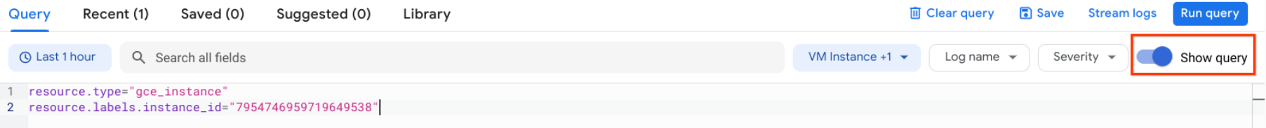
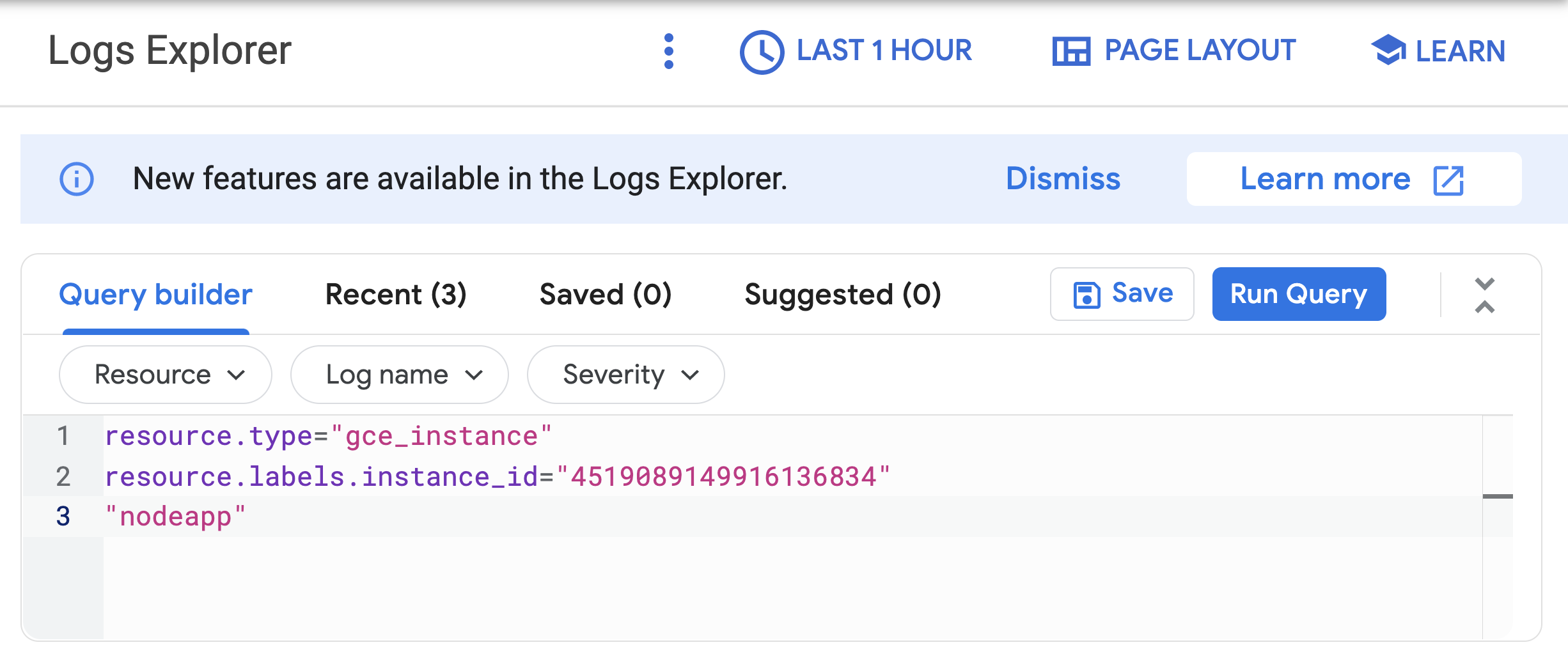
  1. Select Navigation menu > Logging > Logs Explorer.
  2. Select the logs you want to see, in this case, you select the logs for the lamp-1-vm instance you created at the start of this lab:
    • Click on Resource.
    • Select VM Instance > lamp-1-vm in the Resource drop-down menu.
    • Click Apply.
    • Leave the other fields with their default values.
    • Click the Stream logs.

You see the logs for your VM instance.

Check out what happens when you start and stop the VM instance.

To best see how Cloud Monitoring and Cloud Logging reflect VM instance changes, make changes to your instance in one browser window and then see what happens in the Cloud Monitoring, and then Cloud Logging windows.

  1. Open the Compute Engine window in a new browser window. Select Navigation menu > Compute Engine, right-click VM instances > Open link in new window.
  2. Move the Logs Viewer browser window next to the Compute Engine window. This makes it easier to view how changes to the VM are reflected in the logs
  3. In the Compute Engine window, select the lamp-1-vm instance, click the three vertical dots at the right of the screen and then click Stop, and then confirm to stop the instance.It takes a few minutes for the instance to stop.
  4. Watch in the Logs View tab for when the VM is stopped.
  5. In the VM instance details window, click the three vertical dots at the right of the screen and then click Start/resume, and then confirm. It will take a few minutes for the instance to re-start. Watch the log messages to monitor the start up.

Task 7. Check the uptime check results and triggered alerts

  1. In the Cloud Logging window, select Navigation menu > Monitoring > Uptime checks. This view provides a list of all active uptime checks, and the status of each in different locations.You will see Lamp Uptime Check listed. Since you have just restarted your instance, the regions are in a failed status. It may take up to 5 minutes for the regions to become active. Reload your browser window as necessary until the regions are active.
  2. Click the name of the uptime check, Lamp Uptime Check.Since you have just restarted your instance, it may take some minutes for the regions to become active. Reload your browser window as necessary.

Check if alerts have been triggered

  1. In the left menu, click Alerting.
  2. You see incidents and events listed in the Alerting window.
  3. Check your email account. You should see Cloud Monitoring Alerts.

Note: Remove the email notification from your alerting policy. The resources for the lab may be active for a while after you finish, and this may result in a few more email notifications getting sent out.

Congratulations! You have successfully set up and monitored a VM with Cloud Monitoring on GCP.

Setting Up Cost Control with Quota

In this lab you will complete the following tasks:

  • Queried a public dataset and explore associated costs.
  • Modified BigQuery API quota.
  • Tried to rerun the query after quota had been modified.

Activate Cloud Shell

Cloud Shell is a virtual machine that is loaded with development tools. It offers a persistent 5GB home directory and runs on the Google Cloud. Cloud Shell provides command-line access to your Google Cloud resources.

  1. Click Activate Cloud Shell Activate Cloud Shell icon at the top of the Google Cloud console.

When you are connected, you are already authenticated, and the project is set to your PROJECT_ID. The output contains a line that declares the PROJECT_ID for this session: Your Cloud Platform project in this session is set to YOUR_PROJECT_ID

gcloud is the command-line tool for Google Cloud. It comes pre-installed on Cloud Shell and supports tab completion.

  1. (Optional) You can list the active account name with this command:

gcloud auth list

  1. Click Authorize.

Open the BigQuery console

  1. In the Google Cloud Console, select Navigation menu > BigQuery.

The Welcome to BigQuery in the Cloud Console message box opens. This message box links the quickstart guide and the release notes.

  1. Click Done.

The BigQuery console opens.

Task 1. Query a public dataset in BigQuery

In this lab, you query the bigquery-public-data:wise_all_sky_data_release public dataset. Learn more about this dataset from the blog post Querying the Stars with BigQuery GIS.

  1. In the Query editor paste the following query:SELECT w1mpro_ep, mjd, load_id, frame_id FROM `bigquery-public-data.wise_all_sky_data_release.mep_wise` ORDER BY mjd ASC LIMIT 500
  2. Do not run the query. Instead, please answer the following question:

Use the query validator to determine how many bytes of data this will process when you run.

  1. Now run the query and see how quickly BigQuery processes that size of data.

Task 2. Explore query cost

The first 1 TB of query data processed per month is free.

Task 3. Update BigQuery quota

In this task, you update the BigQuery API quota to restrict the data processed in queries in your project.

  1. In your Cloud Shell, run this command to view your current usage quotas with the BigQuery API:

gcloud alpha services quota list –service=bigquery.googleapis.com –consumer=projects/${DEVSHELL_PROJECT_ID} –filter=”usage”

The consumerQuotaLimits display your current query per day limits. There is a separate quota for usage per project and usage per user.

  1. Run this command in Cloud Shell to update your per user quota to .25 TiB per day:

gcloud alpha services quota update –consumer=projects/${DEVSHELL_PROJECT_ID} –service bigquery.googleapis.com –metric bigquery.googleapis.com/quota/query/usage –value 262144 –unit 1/d/{project}/{user} –force

  1. After the quota is updated, examine your consumerQuotaLimits again:

gcloud alpha services quota list –service=bigquery.googleapis.com –consumer=projects/${DEVSHELL_PROJECT_ID} –filter=”usage”

You should see the same limits from before but also a consumerOverride with the value used in the previous step:— consumerQuotaLimits: – metric: bigquery.googleapis.com/quota/query/usage quotaBuckets: – defaultLimit: ‘9223372036854775807’ effectiveLimit: ‘9223372036854775807’ unit: 1/d/{project} – metric: bigquery.googleapis.com/quota/query/usage quotaBuckets: – consumerOverride: name:projects/33699896259/services/bigquery.googleapis.com/consumerQuotaMetrics/bigquery.googleapis.com%2Fquota%2Fquery%2Fusage/limits/%2Fd%2Fproject%2Fuser/consumerOverrides/Cg1RdW90YU92ZXJyaWRl overrideValue: ‘262144’ defaultLimit: ‘9223372036854775807’ effectiveLimit: ‘262144’ unit: 1/d/{project}/{user} displayName: Query usage metric: bigquery.googleapis.com/quota/query/usage unit: MiBy

Next, you will re-run your query with the updated quota.

Task 4. Rerun your query

  1. In the Cloud Console, click BigQuery.
  2. The query you previously ran should still be in the query editor, but if it isn’t, paste the following query in the Query editor and click Run: SELECT w1mpro_ep, mjd, load_id, frame_id FROM `bigquery-public-data.wise_all_sky_data_release.mep_wise` ORDER BY mjd ASC LIMIT 500
  3. Note the validator still mentions This query will process 1.36 TB when run. However, the query has run successfully and hasn’t processed any data. Why do you think that is?

Running the same query again may not process any data because of the automatic query, Caching feature in BigQuery.ShufflingJoiningcheck

Note: If your query is already blocked by your custom quota, don’t worry. It’s likely that you set the custom quota and re-run the query before the first query had time to cache the results.

Queries that use cached query results are at no additional charge and do not count against your quota. For more information on using cached query results, see Using cached query results.

In order for us to test the newly set quota, you must to disable query cache to process data using the previous query.

  1. To test that the quota has changed, disable the cached query results. In the Query results pane, click More > Query settings:
Query settings option highlighted in the More dropdown mnenu
  1. Uncheck Use cached results and click Save.
  2. Run the query again so that it counts against your daily quota.
  3. Once the query has run successfully and processed the 1.36 TB, run the query once more.What happened? Were you able to run the query? You should have received an error like the following:Custom quota exceeded: Your usage exceeded the custom quota for QueryUsagePerUserPerDay, which is set by your administrator. For more information, see https://cloud.google.com/bigquery/cost-controls

Task 5. Explore BigQuery best practices

Quotas can be used for cost controls but it’s up to your business to determine which quotas make sense for your team. This is one example of how to set quotas to protect from unexpected costs. One way to reduce the amount of data queried is to optimize your queries.

Learn more about optimizing BigQuery queries from the Control costs in BigQuery guide.

And just like that you completed all the tasks! Congrats..

Distributed Load Testing Using Kubernetes

Activate Cloud Shell

Cloud Shell is a virtual machine that is loaded with development tools. It offers a persistent 5GB home directory and runs on the Google Cloud. Cloud Shell provides command-line access to your Google Cloud resources.

  1. Click Activate Cloud Shell Activate Cloud Shell icon at the top of the Google Cloud console.

When you are connected, you are already authenticated, and the project is set to your PROJECT_ID. The output contains a line that declares the PROJECT_ID for this session:Your Cloud Platform project in this session is set to YOUR_PROJECT_ID

gcloud is the command-line tool for Google Cloud. It comes pre-installed on Cloud Shell and supports tab-completion.

  1. (Optional) You can list the active account name with this command:

gcloud auth list

  1. Click Authorize.

Task 1. Set project and zone

  • Define environment variables for the project idregion and zone you want to use for the lab.

PROJECT=$(gcloud config get-value project) REGION=us-central1 ZONE=${REGION}-a CLUSTER=gke-load-test TARGET=${PROJECT}.appspot.com gcloud config set compute/region $REGION gcloud config set compute/zone $ZONE

Task 2. Get the sample code and build a Docker image for the application

  1. Get the source code from the repository by running:

gsutil -m cp -r gs://spls/gsp182/distributed-load-testing-using-kubernetes .

  1. Move into the directory:

cd distributed-load-testing-using-kubernetes/

  1. Build docker image and store it in container registry:

gcloud builds submit –tag gcr.io/$PROJECT/locust-tasks:latest docker-image/.

Example Output:ID CREATE_TIME DURATION SOURCE IMAGES STATUS 47f1b8f7-0b81-492c-aa3f-19b2b32e515d xxxxxxx 51S gs://project_id_cloudbuild/source/1554261539.12-a7945015d56748e796c55f17b448e368.tgz gcr.io/project_id/locust-tasks (+1 more) SUCCESS

Task 3. Deploy web application

The sample-webapp folder contains a simple Google App Engine Python application as the “system under test”.

  • To deploy the application to your project use the gcloud app deploy command:

gcloud app deploy sample-webapp/app.yaml

After running the command, you’ll be prompted with the following.Please choose the region where you want your App Engine application located:

From the list of regions, you can choose us-central, since we selected us-central1 as the region for this project. To choose us-central enter “10” as the input for the prompt.Please enter your numeric choice: 10Note: You will need the URL of the deployed sample web application when deploying the locust-master and locust-worker deployments which is already stored in TARGET variable.

Task 4. Deploy Kubernetes cluster

gcloud container clusters create $CLUSTER \ –zone $ZONE \ –num-nodes=5

Example output:NAME: gke-load-test LOCATION: us-central1-a MASTER_VERSION: 1.11.7-gke.12 MASTER_IP: 34.66.156.246 MACHINE_TYPE: n1-standard-1 NODE_VERSION: 1.11.7-gke.12 NUM_NODES: 5 STATUS: RUNNING

Task 5. Load testing master

The first component of the deployment is the Locust master, which is the entry point for executing the load testing tasks described above. The Locust master is deployed with a single replica because we need only one master.

The configuration for the master deployment specifies several elements, including the ports that need to be exposed by the container (8089 for web interface, 5557 and 5558 for communicating with workers). This information is later used to configure the Locust workers.

The following snippet contains the configuration for the ports:ports: – name: loc-master-web containerPort: 8089 protocol: TCP – name: loc-master-p1 containerPort: 5557 protocol: TCP – name: loc-master-p2 containerPort: 5558 protocol: TCP

Task 6. Deploy locust-master

  1. Replace [TARGET_HOST] and [PROJECT_ID] in locust-master-controller.yaml and locust-worker-controller.yaml with the deployed endpoint and project-id respectively.

sed -i -e “s/\[TARGET_HOST\]/$TARGET/g” kubernetes-config/locust-master-controller.yaml sed -i -e “s/\[TARGET_HOST\]/$TARGET/g” kubernetes-config/locust-worker-controller.yaml sed -i -e “s/\[PROJECT_ID\]/$PROJECT/g” kubernetes-config/locust-master-controller.yaml sed -i -e “s/\[PROJECT_ID\]/$PROJECT/g” kubernetes-config/locust-worker-controller.yaml

  1. Deploy Locust master:

kubectl apply -f kubernetes-config/locust-master-controller.yaml

  1. To confirm that the locust-master pod is created, run the following command:

kubectl get pods -l app=locust-master

  1. Next, deploy the locust-master-service:

kubectl apply -f kubernetes-config/locust-master-service.yaml

This step will expose the pod with an internal DNS name (locust-master) and ports 80895557, and 5558. As part of this step, the type: LoadBalancer directive in locust-master-service.yaml will tell Google Kubernetes Engine to create a Compute Engine forwarding-rule from a publicly available IP address to the locust-master pod.

  1. To view the newly created forwarding-rule, execute the following:

kubectl get svc locust-master

Example output:NAME TYPE CLUSTER-IP EXTERNAL-IP PORT(S) AGE locust-master LoadBalancer 10.59.244.88 35.222.161.198 8089:30865/TCP,5557:30707/TCP,5558:31327/TCP 1m

Task 7. Load testing workers

The next component of the deployment includes the Locust workers, which execute the load testing tasks described above. The Locust workers are deployed by a single deployment that creates multiple pods. The pods are spread out across the Kubernetes cluster. Each pod uses environment variables to control important configuration information such as the hostname of the system under test and the hostname of the Locust master.

After the Locust workers are deployed, you can return to the Locust master web interface and see that the number of slaves corresponds to the number of deployed workers.

The following snippet contains the deployment configuration for the name, labels, and number of replicas:apiVersion: “apps/v1” kind: “Deployment” metadata: name: locust-worker labels: name: locust-worker spec: replicas: 5 selector: matchLabels: app: locust-worker template: metadata: labels: app: locust-worker spec: …

Deploy locust-worker

  1. Now deploy locust-worker-controller:

kubectl apply -f kubernetes-config/locust-worker-controller.yaml

  1. The locust-worker-controller is set to deploy 5 locust-worker pods. To confirm they were deployed, run the following:

kubectl get pods -l app=locust-worker

Scaling up the number of simulated users will require an increase in the number of Locust worker pods. To increase the number of pods deployed by the deployment, Kubernetes offers the ability to resize deployments without redeploying them.

  1. The following command scales the pool of Locust worker pods to 20:

kubectl scale deployment/locust-worker –replicas=20

  1. To confirm that pods have launched and are ready, get the list of locust-worker pods:

kubectl get pods -l app=locust-worker

The following diagram shows the relationship between the Locust master and the Locust workers:

The flow from the Locust master to the Locust worker to the application

Task 8. Execute tests

  1. To execute the Locust tests, get the external IP address by following command:

EXTERNAL_IP=$(kubectl get svc locust-master -o yaml | grep ip: | awk -F”: ” ‘{print $NF}’) echo http://$EXTERNAL_IP:8089

  1. Click the link and navigate to Locust master web interface.

The Locust master web interface enables you to execute the load testing tasks against the system under test.

934dc685f86ood1f.png
  1. To begin, specify the total number of users to simulate and a rate at which each user should be spawned.
  2. Next, click Start swarming to begin the simulation. For example you can specify number of users as 300 and rate as 10.
  3. Click Start swarming.

As time progresses and users are spawned, statistics aggregate for simulation metrics, such as the number of requests and requests per second.

  1. To stop the simulation, click Stop and the test will terminate. The complete results can be downloaded into a spreadsheet.

Congratulations! You used Kubernetes Engine to deploy a distributed load testing framework.

Deploying Memcached on Kubernetes Engine

Overview

In this lab, you’ll learn how to deploy a cluster of distributed Memcached servers on Kubernetes Engine using Kubernetes, Helm, and Mcrouter. Memcached is one of the most popular open-source, multi-purpose caching systems. It usually serves as a temporary store for frequently used data to speed up web applications and lighten database loads.

What you’ll learn

  • Learn about some characteristics of Memcached’s distributed architecture.
  • Deploy a Memcached service to Kubernetes Engine using Kubernetes and Helm.
  • Deploy Mcrouter, an open source Memcached proxy, to improve the system’s performance.

Memcached’s characteristics

Memcached has two main design goals:

  • Simplicity: Memcached functions like a large hash table and offers a simple API to store and retrieve arbitrarily shaped objects by key.
  • Speed: Memcached holds cache data exclusively in random-access memory (RAM), making data access extremely fast.

Memcached is a distributed system that allows its hash table capacity to scale horizontally across a pool of servers. Each Memcached server operates in complete isolation from the other servers in the pool. Therefore, the routing and load balancing between the servers must be done at the client level. Memcached clients apply a consistent hashing scheme to appropriately select the target servers. This scheme guarantees the following conditions:

  • The same server is always selected for the same key.
  • Memory usage is evenly balanced between the servers.
  • A minimum number of keys are relocated when the pool of servers is reduced or expanded.

The following diagram illustrates at a high level the interaction between a Memcached client and a distributed pool of Memcached servers.

Memcached client-server interaction diagram

Setup and requirements

Activate Cloud Shell

Cloud Shell is a virtual machine that is loaded with development tools. It offers a persistent 5GB home directory and runs on the Google Cloud. Cloud Shell provides command-line access to your Google Cloud resources.

  1. Click Activate Cloud Shell Activate Cloud Shell icon at the top of the Google Cloud console.

When you are connected, you are already authenticated, and the project is set to your PROJECT_ID. The output contains a line that declares the PROJECT_ID for this session: Your Cloud Platform project in this session is set to YOUR_PROJECT_ID

gcloud is the command-line tool for Google Cloud. It comes pre-installed on Cloud Shell and supports tab completion.

  1. (Optional) You can list the active account name with this command:

gcloud auth list

  1. ClickĀ Authorize.

Task 1. Deploying a Memcached service

A simple way to deploy a Memcached service to Kubernetes Engine is to use a Helm chart.

  • In Cloud Shell, create a new Kubernetes Engine cluster of three nodes:

gcloud container clusters create demo-cluster –num-nodes 3 –zone us-central1-f

This deployment will take between five and ten minutes to complete. You may see a warning about default scopes that you can safely ignore as it has no impact on this lab.Note: The cluster’s zone specified here is arbitrary. You can select another zone for your cluster from the available zones.

Configure Helm

Helm is a package manager that makes it easy to configure and deploy Kubernetes applications. Your Cloud Shell will already have a recent, stable version of Helm pre-installed.

If curious, you can run helm version in Cloud Shell to check which version you are using and also ensure that Helm is installed.

  1. Add Helm’s stable chart repository:

helm repo add stable https://charts.helm.sh/stable

  1. Update the repo to ensure you get the latest list of charts:

helm repo update

  1. Install a new Memcached Helm chart release with three replicas, one for each node:

helm install mycache stable/memcached –set replicaCount=3

The Memcached Helm chart uses a StatefulSet controller. One benefit of using a StatefulSet controller is that the pods’ names are ordered and predictable. In this case, the names are mycache-memcached-{0..2}. This ordering makes it easier for Memcached clients to reference the servers.Note: If you get: “Error: could not find a ready tiller pod.” wait a few seconds and retry the Helm install command. The tiller pod may not have had time to initialize.

  1. Execute the following command to see the running pods:

kubectl get pods

Resulting output:NAME READY STATUS RESTARTS AGE mycache-memcached-0 1/1 Running 0 45s mycache-memcached-1 1/1 Running 0 35s mycache-memcached-2 1/1 Running 0 25s

You may need to run the previous command again to see all three pods in the Ready 1/1 status.

Discovering Memcached service endpoints

The Memcached Helm chart uses a headless service. A headless service exposes IP addresses for all of its pods so that they can be individually discovered.

  1. Verify that the deployed service is headless:

kubectl get service mycache-memcached -o jsonpath=”{.spec.clusterIP}” ; echo

The output None confirms that the service has no clusterIP and that it is therefore headless.

  1. In this lab the service creates a DNS record for a hostname of the form:

[SERVICE_NAME].[NAMESPACE].svc.cluster.local

In this lab the service name is mycache-memcached. Because a namespace was not explicitly defined, the default namespace is used, and therefore the entire hostname is mycache-memcached.default.svc.cluster.local. This hostname resolves to a set of IP addresses and domains for all three pods exposed by the service. If, in the future, some pods get added to the pool, or old ones get removed, kube-dns will automatically update the DNS record.

It is the client’s responsibility to discover the Memcached service endpoints. To do that:

  1. Retrieve the endpoints’ IP addresses:

kubectl get endpoints mycache-memcached

The output is similar to the following:NAME ENDPOINTS AGE mycache-memcached 10.36.0.32:11211,10.36.0.33:11211,10.36.1.25:11211 3m

Notice that each Memcached pod has a separate IP address. These IP addresses might differ for your own server instances. Each pod listens to port 11211, which is Memcached’s default port.

There are a number of alternative methods that can be used such as these two optional examples. You can carry out these steps if you have time, or move directly to the next step where you test the deployment using telnet:

Note – alternate methods: You can retrieve those same records using a standard DNS query with the nslookup command:kubectl run -it –rm alpine –image=alpine:3.6 –restart=Never nslookup mycache-memcached.default.svc.cluster.local

The output is similar to the following:Name: mycache-memcached.default.svc.cluster.local Address 1: 10.0.0.8 mycache-memcached-0.mycache-memcached.default.svc.cluster.local Address 2: 10.0.1.5 mycache-memcached-2.mycache-memcached.default.svc.cluster.local Address 3: 10.0.2.3 mycache-memcached-1.mycache-memcached.default.svc.cluster.local pod “alpine” deleted

Note: You can ignore the nslookup: can't resolve '(null)': Name does not resolve flag if it shows up. Notice that each server has its own domain name of the following form:[POD_NAME].[SERVICE_NAME].[NAMESPACE].svc.cluster.local

For example, the domain for the mycache-memcached-0 pod is: Mycache-memcached-0.mycache-memcached.default.svc.cluster.local

Note: For another alternative approach, you can perform the same DNS inspection by using a programming language like Python.

  1. Start a Python interactive console inside your cluster:

kubectl run -it –rm python –image=python:3.6-alpine –restart=Never python

  1. In the Python console, run these commands:

import socket

print(socket.gethostbyname_ex(‘mycache-memcached.default.svc.cluster.local’))

Note: It takes a while for the pod to get deleted, please wait.Note: The output is similar to the following and is echoed to the console before the exit() command:('mycache-memcached.default.svc.cluster.local', ['mycache-memcached.default.svc.cluster.local'], ['10.36.0.32', '10.36.0.33', '10.36.1.25'])

  1. Test the deployment by opening a telnet session with one of the running Memcached servers on port 11211:

kubectl run -it –rm alpine –image=alpine:3.6 –restart=Never telnet mycache-memcached-0.mycache-memcached.default.svc.cluster.local 11211

This will open a session to the telnet interface with no obvious prompt. Don’t mind the If you don't see a command prompt, try pressing enter–you can start plugging in commands right away (even if the formatting looks a little off.)

At the telnet prompt run these commands using the Memcached ASCII protocol to confirm that telnet is actually connected to a Memcached server instance. As this is a telnet session, enter each set of commands and wait for the response to avoid getting commands and responses mixed on the console.

  1. Store the key:

set mykey 0 0 5 hello

Press Enter and you will see the response:

STORED

  1. Retrieve the key:

get mykey

Press Enter and you will see the response:

VALUE mykey 0 5 hello END

  1. Quit the telnet session:

quit

Press Enter to close the session if it does not automatically exit.

Note: It takes a while for the pod to get deleted, please wait.

Task 2. Implementing the service discovery logic

You are now ready to implement the basic service discovery logic shown in the following diagram.

Basic service discovery logic diagram

At a high level, the service discovery logic consists of the following steps:

  1. The application queries kube-dns for the DNS record of mycache-memcached.default.svc.cluster.local.
  2. The application retrieves the IP addresses associated with that record.
  3. The application instantiates a new Memcached client and provides it with the retrieved IP addresses.
  4. The Memcached client’s integrated load balancer connects to the Memcached servers at the given IP addresses.

Implement the service discovery logic

You now implement this service discovery logic by using Python.

  1. Deploy a new Python-enabled pod in your cluster and start a shell session inside the pod:

kubectl run -it –rm python –image=python:3.6-alpine –restart=Never sh

  1. Once you get a shell prompt (/ #) install the pymemcache library:

pip install pymemcache

  1. Start a Python interactive console by running the python command.

python

  1. In the Python console (>>>), run the following:

import socket from pymemcache.client.hash import HashClient _, _, ips = socket.gethostbyname_ex(‘mycache-memcached.default.svc.cluster.local’) servers = [(ip, 11211) for ip in ips] client = HashClient(servers, use_pooling=True) client.set(‘mykey’, ‘hello’) client.get(‘mykey’)

Note: If you are getting the error SyntaxError: multiple statements found while compiling a single statement then run the above command line by line.

The output that results from the last command:b’hello’

The b prefix signifies a bytes literal, which is the format in which Memcached stores data.

  1. Exit the Python console:

exit()

Exit the pod’s shell session by pressing Control+D.

Task 3. Enabling connection pooling

As your caching needs grow, and the pool scales up to dozens, hundreds, or thousands of Memcached servers, you might run into some limitations. In particular, the large number of open connections from Memcached clients might place a heavy load on the servers, as the following diagram shows.

Memcached client-server open connections diagram

To reduce the number of open connections, you must introduce a proxy to enable connection pooling, as in the following diagram.

Proxy between client and server connections

Mcrouter (pronounced “mick router”), a powerful open source Memcached proxy, enables connection pooling. Integrating Mcrouter is seamless, because it uses the standard Memcached ASCII protocol. To a Memcached client, Mcrouter behaves like a normal Memcached server. To a Memcached server, Mcrouter behaves like a normal Memcached client.

Deploy Mcrouter

To deploy Mcrouter, run the following commands in Cloud Shell.

  1. Uninstall the previously installed mycache Helm chart release:

helm delete mycache

Outputrelease “mycache” uninstalled

  1. Deploy new Memcached pods and Mcrouter pods by installing a new Mcrouter Helm chart release:

helm install mycache stable/mcrouter –set memcached.replicaCount=3

  1. Check the status of the sample application deployment:

kubectl get pods

Repeat the kubectl get pods command periodically until all 3 of the mycache-mcrouter pods report a STATUS of Running and a READY state of 1/1. This may take a couple of minutes. Three mycache-memcached pods are also started by this command and they will initialize first, however you must wait for the mycache-mcrouter pods to be fully ready before proceeding or the pod ip-addresses will not be configured.

Once you see the READY state of 1/1 the mycache-mcrouter proxy pods are now ready to accept requests from client applications.

  1. Test this setup by connecting to one of the proxy pods. Use the telnet command on port 5000, which is Mcrouter’s default port.

MCROUTER_POD_IP=$(kubectl get pods -l app=mycache-mcrouter -o jsonpath=”{.items[0].status.podIP}”)

kubectl run -it –rm alpine –image=alpine:3.6 –restart=Never telnet $MCROUTER_POD_IP 5000

This will open a session to the telnet interface with no obvious prompt. It’ll be ready right away.

In the telnet prompt, run these commands to test the Mcrouter configuration:

  1. Store a key:

set anotherkey 0 0 15 Mcrouter is fun

  1. Press ENTER and you will see the response:

STORED

  1. Retrieve the key:

get anotherkey

  1. Press ENTER and you will see the response:

VALUE anotherkey 0 15 Mcrouter is fun END

  1. Quit the telnet session.

quit

You have now deployed a proxy that enables connection pooling.

Task 4. Reducing latency

To increase resilience, it is common practice to use a cluster with multiple nodes. This lab uses a cluster with three nodes. However, using multiple nodes also brings the risk of increased latency caused by heavier network traffic between nodes.

Colocating proxy pods

You can reduce the latency risk by connecting client application pods only to a Memcached proxy pod that is on the same node. The following diagram illustrates this configuration which shows the topology for the interactions between application pods, Mcrouter pods, and Memcached pods across a cluster of three nodes.

Interaction topology between nodes 1, 2, and 3

In a production environment, you would create this configuration as follows:

  1. Ensure that each node contains one running proxy pod. A common approach is to deploy the proxy pods with a DaemonSet controller. As nodes are added to the cluster, new proxy pods are automatically added to them. As nodes are removed from the cluster, those pods are garbage-collected. In this lab, the Mcrouter Helm chart that you deployed earlier uses a DaemonSet controller by default. So this step is already complete.
  2. Set a hostPort value in the proxy container’s Kubernetes parameters to make the node listen to that port and redirect traffic to the proxy. In this lab, the Mcrouter Helm chart uses this parameter by default for port 5000. So this step is also already complete.
  3. Expose the node name as an environment variable inside the application pods by using the spec.env entry and selecting the spec.nodeName fieldRef value. See more about this method in the Kubernetes documentation. You will perform this step in the next section.

Configure application pods to expose the Kubernetes node name as an environment variable

  1. Deploy some sample application pods with the NODE_NAME environment variable configured to contain the Kubernetes node name by entering the following in the Google Cloud Shell:

cat <<EOF | kubectl create -f – apiVersion: apps/v1 kind: Deployment metadata: name: sample-application-py spec: replicas: 5 selector: matchLabels: app: sample-application-py template: metadata: labels: app: sample-application-py spec: containers: – name: python image: python:3.6-alpine command: [ “sh”, “-c”] args: – while true; do sleep 10; done; env: – name: NODE_NAME valueFrom: fieldRef: fieldPath: spec.nodeName EOF

  1. Enter the following command to check the status of the sample application-py deployment:

kubectl get pods

  1. Repeat the kubectl get pods command until all 5 of the sample-application pods report a Status of Running and a READY state of 1/1. This may take a minute or two.
  1. Verify that the node name is exposed to each pod, by looking inside one of the sample application pods:

POD=$(kubectl get pods -l app=sample-application-py -o jsonpath=”{.items[0].metadata.name}”) kubectl exec -it $POD — sh -c ‘echo $NODE_NAME’

You will see the node’s name in the output in the following form:gke-demo-cluster-default-pool-XXXXXXXX-XXXX

Connecting the pods

The sample application pods are now ready to connect to the Mcrouter pod that runs on their respective mutual nodes at port 5000, which is Mcrouter’s default port.

  1. Use the node name that was outputted when you ran the previous command (kubectl exec -it $POD -- sh -c 'echo $NODE_NAME) and use it in the following to initiate a connection for one of the pods by opening a telnet session:

kubectl run -it –rm alpine –image=alpine:3.6 –restart=Never telnet gke-demo-cluster-default-pool-XXXXXXXX-XXXX 5000

Remember, telnet prompts aren’t obvious, so you can start plugging commands in right away.

  1. In the telnet prompt, run these commands:

get anotherkey

This command outputs the value of this key that we set on the memcached cluster using Mcrouter in the previous section:VALUE anotherkey 0 15 Mcrouter is fun END

  1. Quit the telnet session.

quit

Finally, to demonstrate using code:

  1. Open up a shell on one of the application nodes and prepare an interactive Python session.

kubectl exec -it $POD — sh

pip install pymemcache

python

On the Python command line, enter the following Python commands that set and retrieve a key value using the NODE_NAME environment variable to locate the Mcrouter node from the application’s environment. This variable was set in the sample application configuration.

import os from pymemcache.client.base import Client NODE_NAME = os.environ[‘NODE_NAME’] client = Client((NODE_NAME, 5000)) client.set(‘some_key’, ‘some_value’) result = client.get(‘some_key’) result

You will see output similar to:b’some_value’

  1. Finally retrieve the key value you set earlier:

result = client.get(‘anotherkey’) result

You will see output similar to:b’Mcrouter is fun’

  1. Exit the Python interactive console

exit()

  1. Then press Control+D to close the shell to the sample application pod.

Congratulations!

You have now completed the Deploying Memcached on Kubernetes Engine lab.

Autoscaling an Instance Group with Custom Cloud Monitoring Metrics

Overview

Here, we will create a Compute Engine managed instance group that autoscale based on the value of a custom Cloud Monitoring metric.

What you’ll learn

  • Deploy an autoscaling Compute Engine instance group.
  • Create a custom metric used to scale the instance group.
  • Use the Cloud Console to visualize the custom metric and instance group size.

Application Architecture

The autoscaling application uses a Node.js script installed on Compute Engine instances. The script reports a numeric value to a Cloud monitoring metric. You do not need to know Node.js or JavaScript for this lab. In response to the value of the metric, the application autoscale the Compute Engine instance group up or down as needed.

The Node.js script is used to seed a custom metric with values that the instance group can respond to. In a production environment, you would base autoscaling on a metric that is relevant to your use case.

The application includes the following components:

  1. Compute Engine instance template – A template used to create each instance in the instance group.
  2. Cloud Storage – A bucket used to host the startup script and other script files.
  3. Compute Engine startup script – A startup script that installs the necessary code components on each instance. The startup script is installed and started automatically when an instance starts. When the startup script runs, it in turn installs and starts code on the instance that writes values to the Cloud monitoring custom metric.
  4. Compute Engine instance group – An instance group that autoscale based on the Cloud monitoring metric values.
  5. Compute Engine instances – A variable number of Compute Engine instances.
  6. Custom Cloud Monitoring metric – A custom monitoring metric used as the input value for Compute Engine instance group autoscaling.
Lab architecture diagram

Task 1. Creating the application

Creating the autoscaling application requires downloading the necessary code components, creating a managed instance group, and configuring autoscaling for the managed instance group.

Uploading the script files to Cloud Storage

During autoscaling, the instance group will need to create new Compute Engine instances. When it does, it creates the instances based on an instance template. Each instance needs a startup script. Therefore, the template needs a way to reference the startup script. Compute Engine supports using Cloud Storage buckets as a source for your startup script. In this section, you will make a copy of the startup script and application files for a sample application used by this lab that pushes a pattern of data into a custom Cloud logging metric that you can then use to configure as the metric that controls the autoscaling behavior for an autoscaling group.

Note: There is a pre-existing instance template and group that has been created automatically by the lab that is already running. Autoscaling requires at least 30 minutes to demonstrate both scale-up and scale-down behavior, and you will examine this group later to see how scaling is controlled by the variations in the custom metric values generated by the custom metric scripts.

Task 2. Create a bucket

  1. In the Cloud Console, scroll down to Cloud Storage from the Navigation menu, then click Create.
  2. Give your bucket a unique name, but don’t use a name you might want to use in another project. For details about how to name a bucket, see the bucket naming guidelines. This bucket will be referenced as YOUR_BUCKET throughout the lab.
  3. Accept the default values then click Create.

Click Confirm for Public access will be prevented pop-up if prompted.

When the bucket is created, the Bucket details page opens.

  1. Next, run the following command in Cloud Shell to copy the startup script files from the lab default Cloud Storage bucket to your Cloud Storage bucket. Remember to replace <YOUR BUCKET> with the name of the bucket you just made:

gsutil cp -r gs://spls/gsp087/* gs://<YOUR BUCKET>

  1. After you upload the scripts, click Refresh on the Bucket details page. Your bucket should list the added files.

Understanding the code components

  • Startup.sh – A shell script that installs the necessary components to each Compute Engine instance as the instance is added to the managed instance group.
  • writeToCustomMetric.js – A Node.js snippet that creates a custom monitoring metric whose value triggers scaling. To emulate real-world metric values, this script varies the value over time. In a production deployment, you replace this script with custom code that reports the monitoring metric that you’re interested in, such as a processing queue value.
  • Config.json – A Node.js config file that specifies the values for the custom monitoring metric and is used in writeToCustomMetric.js.
  • Package.json – A Node.js package file that specifies standard installation and dependencies for writeToCustomMetric.js.
  • writeToCustomMetric.sh – A shell script that continuously runs the writeToCustomMetric.js program on each Compute Engine instance.

Task 3. Creating an instance template

Now create a template for the instances that are created in the instance group that will use autoscaling. As part of the template, you specify the location (in Cloud Storage) of the startup script that should run when the instance starts.

  1. In the Cloud Console, click Navigation menu > Compute Engine > Instance templates.
  2. Click Create Instance Template at the top of the page.
  3. Name the instance template autoscaling-instance01.
  4. Scroll down, click Advanced options.
  5. In the Metadata section of the Management tab, enter these metadata keys and values, clicking the + Add item button to add each one. Remember to substitute your bucket name for the [YOUR_BUCKET_NAME] placeholder:
KeyValue
startup-script-urlgs://[YOUR_BUCKET_NAME]/startup.sh
gcs-bucketgs://[YOUR_BUCKET_NAME]
  1. Click Create.

Task 4. Creating the instance group

  1. In the left pane, click Instance groups.
  2. Click Create instance group at the top of the page.
  3. Name: autoscaling-instance-group-1.
  4. For Instance template, select the instance template you just created.
  5. Set Autoscaling mode to Off: do not autoscale.

You’ll edit the autoscaling setting after the instance group has been created. Leave the other settings at their default values.

  1. Click Create.

Note: You can ignore the Autoscaling is turned off. The number of instances in the group won't change automatically. The autoscaling configuration is preserved. warning next to your instance group.

Task 5. Verifying that the instance group has been created

Wait to see the green check mark next to the new instance group you just created. It might take the startup script several minutes to complete installation and begin reporting values. Click Refresh if it seems to be taking more than a few minutes.

Note: If you see a red icon next to the other instance group that was pre-created by the lab, you can ignore this warning. The instance group reports a warning for up to ten minutes as it is initializing. This is expected behavior.

Task 6. Verifying that the Node.js script is running

The custom metric custom.googleapis.com/appdemo_queue_depth_01 isn’t created until the first instance in the group is created and that instance begins reporting custom metric values.

You can verify that the writeToCustomMetric.js script is running on the first instance in the instance group by checking whether the instance is logging custom metric values.

  1. Still in the Compute Engine Instance groups window, click the name of the autoscaling-instance-group-1 to display the instances that are running in the group.
  2. Scroll down and click the instance name. Because autoscaling has not started additional instances, there is just a single instance running.
  3. In the Details tab, in the Logs section, click Cloud Logging link to view the logs for the VM instance.
  4. Wait a minute or 2 to let some data accumulate. Enable the Show query toggle, you will see resource.type and resource.labels.instance_id in the Query preview box.
 Query preview box
  1. Add “nodeapp” as line 3, so the code looks similar to this:
Line 1: resource.type="gce.instance". Line 2: resource.labels.instance_id="4519089149916136834". Line 3: "nodeapp"
  1. Click Run query.

If the Node.js script is being executed on the Compute Engine instance, a request is sent to the API, and log entries that say Finished writing time series data appear in the logs.

Note: If you don’t see this log entry, the Node.js script isn’t reporting the custom metric values. Check that the metadata was entered correctly. If the metadata is incorrect, it might be easiest to restart the lab.

Task 7. Configure autoscaling for the instance group

After you’ve verified that the custom metric is successfully reporting data from the first instance, the instance group can be configured to autoscale based on the value of the custom metric.

  1. In the Cloud Console, go to Compute Engine > Instance groups.
  2. Click the autoscaling-instance-group-1 group.
  3. Under Autoscaling click Configure.
  4. Set Autoscaling mode to On: add and remove instances to the group.
  5. Set Minimum number of instances1 and Maximum number of instances3
  6. Under Autoscaling signals click ADD SIGNAL to edit metric. Set the following fields, leave all others at the default value.
  • Signal typeCloud Monitoring metric new. Click Configure.
  • Under Resource and metric click SELECT A METRIC and navigate to VM Instance > Custom metrics > Custom/appdemo_queue_depth_01.
  • Click Apply.
  • Utilization target150When custom monitoring metric values are higher or lower than the Target value, the autoscaler scales the managed instance group, increasing or decreasing the number of instances. The target value can be any double value, but for this lab, the value 150 was chosen because it matches the values being reported by the custom monitoring metric.
  • Utilization target typeGauge. Click Select.The Gauge setting specifies that the autoscaler should compute the average value of the data collected over the last few minutes and compare it to the target value. (By contrast, setting Target mode to DELTA_PER_MINUTE or DELTA_PER_SECOND autoscales based on the observed rate of change rather than an average value.)
  1. Click Save.

Task 8. Watching the instance group perform autoscaling

The Node.js script varies the custom metric values it reports from each instance over time. As the value of the metric goes up, the instance group scales up by adding Compute Engine instances. If the value goes down, the instance group detects this and scales down by removing instances. As noted earlier, the script emulates a real-world metric whose value might similarly fluctuate up and down.

Next, you will see how the instance group is scaling in response to the metric by clicking the Monitoring tab to view the Autoscaled size graph.

  1. In the left pane, click Instance groups.
  2. Click the builtin-igm instance group in the list.
  3. Click the Monitoring tab.
  4. Enable Auto Refresh.

Since this group had a head start, you can see the autoscaling details about the instance group in the autoscaling graph. The autoscaler will take about five minutes to correctly recognize the custom metric and it can take up to ten minutes for the script to generate sufficient data to trigger the autoscaling behavior.

Monitoring tabbed page displaying two monitoring graphs

Hover your mouse over the graphs to see more details.

You can switch back to the instance group that you created to see how it’s doing (there may not be enough time left in the lab to see any autoscaling on your instance group).

For the remainder of the time in your lab, you can watch the autoscaling graph move up and down as instances are added and removed.

Task 9. Autoscaling example

Read this autoscaling example to see how the capacity and number of autoscaled instances can work in a larger environment.

The number of instances depicted in the top graph changes as a result of the varying aggregate levels of the custom metric property values reported in the lower graph. There is a slight delay of up to five minutes after each instance starts up before that instance begins to report its custom metric values. While your autoscaling starts up, read through this graph to understand what will be happening:

Members tabbed page displaying a graph with several data points

The script starts by generating high values for approximately 15 minutes in order to trigger scale-up behavior.

  • 11:27 Autoscaling Group starts with a single instance. The aggregate custom metric target is 150.
  • 11:31 Initial metric data acquired. As the metric is greater than the target of 150 the autoscaling group starts a second instance.
  • 11:33 Custom metric data from the second instance starts to be acquired. The aggregate target is now 300. As the metric value is above 300 the autoscaling group starts the third instance.
  • 11:37 Custom metric data from the third instance starts to be acquired. The aggregate target is now 450. As the cumulative metric value is above 450 the autoscaling group starts the fourth instance.
  • 11:42 Custom metric data from the fourth instance starts to be acquired. The aggregate target is now 600. The cumulative metric value is now above the new target level of 600 but since the autoscaling group size limit has been reached no additional scale-up actions occur.
  • 11:44 The application script has moved into a low metric 15-minute period. Even though the cumulative metric value is below the target of 600 scale-down must wait for a ten-minute built-in scale-down delay to pass before making any changes.
  • 11:54 Custom metric data has now been below the aggregate target level of 600 for a four-node cluster for over 10 minutes. Scale-down now removes two instances in quick succession.
  • 11:56 Custom metric data from the removed nodes is eliminated from the autoscaling calculation and the aggregate target is reduced to 300.
  • 12:00 The application script has moved back into a high metric 15-minute period. The cumulative custom metric value has risen above the aggregate target level of 300 again so the autoscaling group starts a third instance.
  • 12:03 Custom metric data from the new instance have been acquired but the cumulative values reported remain below the target of 450 so autoscaling makes no changes.
  • 12:04 Cumulative custom metric values rise above the target of 450 so autoscaling starts the fourth instance.

Congratulations!

You have successfully created a managed instance group that autoscale based on the value of a custom metric.

Continuous Delivery Pipelines with Spinnaker and Kubernetes Engine

Overview

This post shows you how to create a continuous delivery pipeline using Google Kubernetes Engine, Google Cloud Source Repositories, Google Cloud Container Builder, and Spinnaker. After you create a sample application, you configure these services to automatically build, test, and deploy it. When you modify the application code, the changes trigger the continuous delivery pipeline to automatically rebuild, retest, and redeploy the new version.

Objectives

  • Set up your environment by launching Google Cloud Shell, creating a Kubernetes Engine cluster, and configuring your identity and user management scheme.
  • Download a sample application, create a Git repository then upload it to a Google Cloud Source Repository.
  • Deploy Spinnaker to Kubernetes Engine using Helm.
  • Build your Docker image.
  • Create triggers to create Docker images when your application changes.
  • Configure a Spinnaker pipeline to reliably and continuously deploy your application to Kubernetes Engine.
  • Deploy a code change, triggering the pipeline, and watch it roll out to production.

Pipeline architecture

To continuously deliver application updates to your users, you need an automated process that reliably builds, tests, and updates your software. Code changes should automatically flow through a pipeline that includes artifact creation, unit testing, functional testing, and production rollout. In some cases, you want a code update to apply to only a subset of your users, so that it is exercised realistically before you push it to your entire user base. If one of these canary releases proves unsatisfactory, your automated procedure must be able to quickly roll back the software changes.

Process diagram

With Kubernetes Engine and Spinnaker you can create a robust continuous delivery flow that helps to ensure your software is shipped as quickly as it is developed and validated. Although rapid iteration is your end goal, you must first ensure that each application revision passes through a gamut of automated validations before becoming a candidate for production rollout. When a given change has been vetted through automation, you can also validate the application manually and conduct further pre-release testing.

After your team decides the application is ready for production, one of your team members can approve it for production deployment.

Application delivery pipeline

In this you will build the continuous delivery pipeline shown in the following diagram.

Continuous delivery pipeline flow diagram

Activate Cloud Shell

Cloud Shell is a virtual machine that is loaded with development tools. It offers a persistent 5GB home directory and runs on the Google Cloud. Cloud Shell provides command-line access to your Google Cloud resources.

  1. Click Activate Cloud Shell Activate Cloud Shell icon at the top of the Google Cloud console.

When connected, you are already authenticated, and the project is set to your PROJECT_ID. The output contains a line that declares the PROJECT_ID for this session: Your Cloud Platform project in this session is set to YOUR_PROJECT_ID

gcloud is the command-line tool for Google Cloud. It comes pre-installed on Cloud Shell and supports tab completion.

  1. (Optional) You can list the active account name with this command:

gcloud auth list

  1. Click Authorize

4. (Optional) You can list the project ID with this command:

gcloud config list project

Task 1. Set up your environment

Configure the infrastructure and identities required for this lab. First you’ll create a Kubernetes Engine cluster to deploy Spinnaker and the sample application.

  1. Set the default compute zone:

gcloud config set compute/zone us-east1-d

  1. Create a Kubernetes Engine cluster using the Spinnaker tutorial sample application:

gcloud container clusters create spinnaker-tutorial \ –machine-type=n1-standard-2

Cluster creation takes between 5 to 10 minutes to complete. Wait for your cluster to finish provisioning before proceeding.

When completed you see a report detailing the name, location, version, ip-address, machine-type, node version, number of nodes and status of the cluster that indicates the cluster is running.

Configure identity and access management

Create a Cloud Identity Access Management (Cloud IAM) service account to delegate permissions to Spinnaker, allowing it to store data in Cloud Storage. Spinnaker stores its pipeline data in Cloud Storage to ensure reliability and resiliency. If your Spinnaker deployment unexpectedly fails, you can create an identical deployment in minutes with access to the same pipeline data as the original.

Upload your startup script to a Cloud Storage bucket by following these steps:

  1. Create the service account:

gcloud iam service-accounts create spinnaker-account \ –display-name spinnaker-account

  1. Store the service account email address and your current project ID in environment variables for use in later commands:

export SA_EMAIL=$(gcloud iam service-accounts list \ –filter=”displayName:spinnaker-account” \ –format=’value(email)’)

export PROJECT=$(gcloud info –format=’value(config.project)’)

  1. Bind the storage.admin role to your service account:

gcloud projects add-iam-policy-binding $PROJECT \ –role roles/storage.admin \ –member serviceAccount:$SA_EMAIL

  1. Download the service account key. In a later step, you will install Spinnaker and upload this key to Kubernetes Engine:

gcloud iam service-accounts keys create spinnaker-sa.json \ –iam-account $SA_EMAIL

Task 2. Set up Cloud Pub/Sub to trigger Spinnaker pipelines

  1. Create the Cloud Pub/Sub topic for notifications from Container Registry:

gcloud pubsub topics create projects/$PROJECT/topics/gcr

  1. Create a subscription that Spinnaker can read from to receive notifications of images being pushed:

gcloud pubsub subscriptions create gcr-triggers \ –topic projects/${PROJECT}/topics/gcr

  1. Give Spinnaker’s service account permissions to read from the gcr-triggers subscription:

export SA_EMAIL=$(gcloud iam service-accounts list \ –filter=”displayName:spinnaker-account” \ –format=’value(email)’)

gcloud beta pubsub subscriptions add-iam-policy-binding gcr-triggers \ –role roles/pubsub.subscriber –member serviceAccount:$SA_EMAIL

Task 3. Deploying Spinnaker using Helm

In this section you use Helm to deploy Spinnaker from the Charts repository. Helm is a package manager you can use to configure and deploy Kubernetes applications.

Helm is already installed in your Cloud Shell.

Configure Helm

  1. Grant Helm the cluster-admin role in your cluster:

kubectl create clusterrolebinding user-admin-binding \ –clusterrole=cluster-admin –user=$(gcloud config get-value account)

  1. Grant Spinnaker the cluster-admin role so it can deploy resources across all namespaces:

kubectl create clusterrolebinding –clusterrole=cluster-admin \ –serviceaccount=default:default spinnaker-admin

  1. Add the stable charts deployments to Helm’s usable repositories (includes Spinnaker):

helm repo add stable https://charts.helm.sh/stable helm repo update

Configure Spinnaker

  1. Still in Cloud Shell, create a bucket for Spinnaker to store its pipeline configuration:

export PROJECT=$(gcloud info \ –format=’value(config.project)’)

export BUCKET=$PROJECT-spinnaker-config

gsutil mb -c regional -l us-east1 gs://$BUCKET

  1. Run the following command to create a spinnaker-config.yaml file, which describes how Helm should install Spinnaker:

export SA_JSON=$(cat spinnaker-sa.json) export PROJECT=$(gcloud info –format=’value(config.project)’) export BUCKET=$PROJECT-spinnaker-config cat > spinnaker-config.yaml <<EOF gcs: enabled: true bucket: $BUCKET project: $PROJECT jsonKey: ‘$SA_JSON’ dockerRegistries: – name: gcr address: https://gcr.io username: _json_key password: ‘$SA_JSON’ email: 1234@5678.com # Disable minio as the default storage backend minio: enabled: false # Configure Spinnaker to enable GCP services halyard: spinnakerVersion: 1.19.4 image: repository: us-docker.pkg.dev/spinnaker-community/docker/halyard tag: 1.32.0 pullSecrets: [] additionalScripts: create: true data: enable_gcs_artifacts.sh: |- \$HAL_COMMAND config artifact gcs account add gcs-$PROJECT –json-path /opt/gcs/key.json \$HAL_COMMAND config artifact gcs enable enable_pubsub_triggers.sh: |- \$HAL_COMMAND config pubsub google enable \$HAL_COMMAND config pubsub google subscription add gcr-triggers \ –subscription-name gcr-triggers \ –json-path /opt/gcs/key.json \ –project $PROJECT \ –message-format GCR EOF

Deploy the Spinnaker chart

  1. Use the Helm command-line interface to deploy the chart with your configuration set:

helm install -n default cd stable/spinnaker -f spinnaker-config.yaml \ –version 2.0.0-rc9 –timeout 10m0s –wait

Note: The installation typically takes 5-8 minutes to complete.

  1. After the command completes, run the following command to set up port forwarding to Spinnaker from Cloud Shell:

export DECK_POD=$(kubectl get pods –namespace default -l “cluster=spin-deck” \ -o jsonpath=”{.items[0].metadata.name}”)

kubectl port-forward –namespace default $DECK_POD 8080:9000 >> /dev/null &

  1. To open the Spinnaker user interface, click the Web Preview icon at the top of the Cloud Shell window and select Preview on port 8080.
Web Preview icon at the top of the Cloud Shell window

The welcome screen opens, followed by the Spinnaker user interface.

Leave this tab open, this is where you’ll access the Spinnaker UI.

Task 4. Building the Docker image

In this section, you configure Cloud Build to detect changes to your app source code, build a Docker image, and then push it to Container Registry.

Create your source code repository

  1. In Cloud Shell tab, download the sample application source code:

gsutil -m cp -r gs://spls/gsp114/sample-app.tar .

  1. Unpack the source code:

mkdir sample-app tar xvf sample-app.tar -C ./sample-app

  1. Change directories to the source code:

cd sample-app

  1. Set the username and email address for your Git commits in this repository. Replace [USERNAME] with a username you create:

git config –global user.email “$(gcloud config get-value core/account)”

Copied!content_copygit config –global user.name “[USERNAME]”

  1. Make the initial commit to your source code repository:

git init

git add .

git commit -m “Initial commit”

  1. Create a repository to host your code:

gcloud source repos create sample-app

Note: Disregard the “you may be billed for this repository” message.git config credential.helper gcloud.sh

  1. Add your newly created repository as remote:

export PROJECT=$(gcloud info –format=’value(config.project)’)

git remote add origin https://source.developers.google.com/p/$PROJECT/r/sample-app

  1. Push your code to the new repository’s master branch:

git push origin master

  1. Check that you can see your source code in the Console by clicking Navigation Menu > Source Repositories.
  2. Click sample-app.

Configure your build triggers

Configure Container Builder to build and push your Docker images every time you push Git tags to your source repository. Container Builder automatically checks out your source code, builds the Docker image from the Dockerfile in your repository, and pushes that image to Google Cloud Container Registry.

Container Builder flow diagram
  1. In the Cloud Platform Console, click Navigation menu > Cloud Build > Triggers.
  2. Click Create trigger.
  3. Set the following trigger settings:
  • Namesample-app-tags
  • Event: Push new tag
  • Select your newly created sample-app repository.
  • Tag.*(any tag)
  • ConfigurationCloud Build configuration file (yaml or json)
  • Cloud Build configuration file location/cloudbuild.yaml
  1. Click CREATE.
CreateTrigger-1.png

From now on, whenever you push a Git tag (.*) to your source code repository, Container Builder automatically builds and pushes your application as a Docker image to Container Registry.

Prepare your Kubernetes Manifests for use in Spinnaker

Spinnaker needs access to your Kubernetes manifests in order to deploy them to your clusters. This section creates a Cloud Storage bucket that will be populated with your manifests during the CI process in Cloud Build. After your manifests are in Cloud Storage, Spinnaker can download and apply them during your pipeline’s execution.

  1. Create the bucket:

export PROJECT=$(gcloud info –format=’value(config.project)’)

gsutil mb -l us-east1 gs://$PROJECT-kubernetes-manifests

  1. Enable versioning on the bucket so that you have a history of your manifests:

gsutil versioning set on gs://$PROJECT-kubernetes-manifests

  1. Set the correct project ID in your kubernetes deployment manifests:

sed -i s/PROJECT/$PROJECT/g k8s/deployments/*

  1. Commit the changes to the repository:

git commit -a -m “Set project ID”

Build your image

Push your first image using the following steps:

  1. In Cloud Shell, still in the sample-app directory, create a Git tag:

git tag v1.0.0

  1. Push the tag:

git push –tags

  1. Go to the Cloud Console. Still in Cloud Build, click History in the left pane to check that the build has been triggered. If not, verify that the trigger was configured properly in the previous section.

Stay on this page and wait for the build to complete before going on to the next section.Note: If the Build fails, then click on the Build ID to open the Build details page and then click RETRY.

Task 5. Configuring your deployment pipelines

Now that your images are building automatically, you need to deploy them to the Kubernetes cluster.

You deploy to a scaled-down environment for integration testing. After the integration tests pass, you must manually approve the changes to deploy the code to production services.

Install the spin CLI for managing Spinnaker

spin is a command-line utility for managing Spinnaker’s applications and pipelines.

  1. Download the 1.14.0 version of spin:

curl -LO https://storage.googleapis.com/spinnaker-artifacts/spin/1.14.0/linux/amd64/spin

  1. Make spin executable:

chmod +x spin

Create the deployment pipeline

  1. Use spin to create an app called sample in Spinnaker. Set the owner email address for the app in Spinnaker:

./spin application save –application-name sample \ –owner-email “$(gcloud config get-value core/account)” \ –cloud-providers kubernetes \ –gate-endpoint http://localhost:8080/gate

Next, you create the continuous delivery pipeline. In this tutorial, the pipeline is configured to detect when a Docker image with a tag prefixed with “v” has arrived in your Container Registry.

  1. From your sample-app source code directory, run the following command to upload an example pipeline to your Spinnaker instance:

export PROJECT=$(gcloud info –format=’value(config.project)’) sed s/PROJECT/$PROJECT/g spinnaker/pipeline-deploy.json > pipeline.json ./spin pipeline save –gate-endpoint http://localhost:8080/gate -f pipeline.json

Manually trigger and view your pipeline execution

The configuration you just created uses notifications of newly tagged images being pushed to trigger a Spinnaker pipeline. In a previous step, you pushed a tag to the Cloud Source Repositories which triggered Cloud Build to build and push your image to Container Registry. To verify the pipeline, manually trigger it.

  1. Switch to your browser tab displaying your Spinnaker UI.

If you are unable to find it, you can get to this tab again by selecting Web Preview > Preview on Port 8080 in your Cloud Shell window.

  1. In the Spinnaker UI, click Applications at the top of the screen to see your list of managed applications.

sample is your application. If you don’t see sample, try refreshing the Spinnaker Applications tab.

  1. Click sample to view your application deployment.
  2. Click Pipelines at the top to view your applications pipeline status.
  3. Click Start Manual Execution, select Deploy in Select Pipeline, and then click Run to trigger the pipeline this first time.
  4. Click Execution Details to see more information about the pipeline’s progress.

The progress bar shows the status of the deployment pipeline and its steps.

Progress bar

Steps in blue are currently running, green ones have completed successfully, and red ones have failed.

  1. Click a stage to see details about it.

After 3 to 5 minutes the integration test phase completes and the pipeline requires manual approval to continue the deployment.

  1. Hover over the yellow “person” icon and click Continue.

Your rollout continues to the production frontend and backend deployments. It completes after a few minutes.

  1. To view the app, at the top of the Spinnaker UI, select Infrastructure > Load Balancers.
  2. Scroll down the list of load balancers and click Default, under service sample-frontend-production. You will see details for your load balancer appear on the right side of the page. If you do not, you may need to refresh your browser.
  3. Scroll down the details pane on the right and copy your app’s IP address by clicking the clipboard button on the Ingress IP. The ingress IP link from the Spinnaker UI may use HTTPS by default, while the application is configured to use HTTP.
Details pane
  1. Paste the address into a new browser tab to view the application. You might see the canary version displayed, but if you refresh you will also see the production version.
Production version of the application

You have now manually triggered the pipeline to build, test, and deploy your application.

Task 6. Triggering your pipeline from code changes

Now test the pipeline end to end by making a code change, pushing a Git tag, and watching the pipeline run in response. By pushing a Git tag that starts with “v”, you trigger Container Builder to build a new Docker image and push it to Container Registry. Spinnaker detects that the new image tag begins with “v” and triggers a pipeline to deploy the image to canaries, run tests, and roll out the same image to all pods in the deployment.

  1. From your sample-app directory, change the color of the app from orange to blue:

sed -i ‘s/orange/blue/g’ cmd/gke-info/common-service.go

  1. Tag your change and push it to the source code repository:

git commit -a -m “Change color to blue”

git tag v1.0.1

git push –tags

  1. In the Console, in Cloud Build > History, wait a couple of minutes for the new build to appear. You may need to refresh your page. Wait for the new build to complete, before going to the next step.

Note: If the Build fails, please click on Build ID and then click RETRY.

  1. Return to the Spinnaker UI and click Pipelines to watch the pipeline start to deploy the image. The automatically triggered pipeline will take a few minutes to appear. You may need to refresh your page.
Pipelines tab in Spinnaker UI

Task 7. Observe the canary deployments

  1. When the deployment is paused, waiting to roll out to production, return to the web page displaying your running application and start refreshing the tab that contains your app. Four of your backends are running the previous version of your app, while only one backend is running the canary. You should see the new, blue version of your app appear about every fifth time you refresh.
  2. When the pipeline completes, your app looks like the following screenshot. Note that the color has changed to blue because of your code change, and that the Version field now reads canary.
Blue canary version

You have now successfully rolled out your app to your entire production environment!

  1. Optionally, you can roll back this change by reverting your previous commit. Rolling back adds a new tag (v1.0.2), and pushes the tag back through the same pipeline you used to deploy v1.0.1:

git revert v1.0.1

Press CTRL+OENTERCTRL+X.git tag v1.0.2

git push –tags

  1. When the build and then the pipeline completes, verify the roll back by clicking Infrastructure > Load Balancers, then click the service sample-frontend-production Default and copy the Ingress IP address into a new tab.

Now your app is back to orange and you can see the production version number.

Orange production version of the UI

Congratulations!

You have now successfully completed the Continuous Delivery Pipelines with Spinnaker and Kubernetes Engine lab.

Setting up Jenkins on Kubernetes Engine on GCP

Activate Cloud Shell

Cloud Shell is a virtual machine that is loaded with development tools. It offers a persistent 5GB home directory and runs on the Google Cloud. Cloud Shell provides command-line access to your Google Cloud resources.

  1. Click Activate Cloud Shell Activate Cloud Shell icon at the top of the Google Cloud console.

When connected, you are already authenticated, and the project is set to your PROJECT_ID. The output contains a line that declares the PROJECT_ID for this session: Your Cloud Platform project in this session is set to YOUR_PROJECT_ID

gcloud is the command-line tool for Google Cloud. It comes pre-installed on Cloud Shell and supports tab completion.

  1. (Optional) You can list the active account name with this command:
gcloud auth list
  1. Click Authorize.
  2. (Optional) You can list the project ID with this command:
gcloud config list project
Output:[core] project = <project_ID>

Task 1. Prepare the environment

First, you’ll prepare your deployment environment and download a sample application.

  1. Set the default Compute Engine zone to <filled in at lab start>:
gcloud config set compute/zone
  1. Clone the sample code:
git clone https://github.com/GoogleCloudPlatform/continuous-deployment-on-kubernetes.git
  1. Navigate to the sample code directory:
cd continuous-deployment-on-kubernetes

Creating a Kubernetes cluster

Now you’ll use the Kubernetes Engine to create and manage your Kubernetes cluster.

  1. Next, provision a Kubernetes cluster using Kubernetes Engine. This step can take several minutes to complete:
gcloud container clusters create jenkins-cd \ --num-nodes 2 \ --scopes "https://www.googleapis.com/auth/projecthosting,cloud-platform"

The extra scopes enable Jenkins to access Cloud Source Repositories and Google Container Registry.

  1. Confirm that your cluster is running:
gcloud container clusters list

Example Output:

Look for RUNNING in the STATUS column:NAME LOCATION MASTER_VERSION MASTER_IP MACHINE_TYPE NODE_VERSION NUM_NODES STATUS jenkins-cd 1.9.7-gke.3 35.237.126.84 e2-medium 1.9.7-gke.3 2 RUNNING

  1. Get the credentials for your cluster. Kubernetes Engine uses these credentials to access your newly provisioned cluster.
gcloud container clusters get-credentials jenkins-cd
  1. Confirm that you can connect to your cluster:
kubectl cluster-info

Example output: If the cluster is running, the URLs of where your Kubernetes components are accessible display:

Kubernetes master is running at https://130.211.178.38 GLBCDefaultBackend is running at https://130.211.178.38/api/v1/proxy/namespaces/kube-system/services/default-http-backendHeapster is running at https://130.211.178.38/api/v1/proxy/namespaces/kube-system/services/heapster KubeDNS is running at https://130.211.178.38/api/v1/proxy/namespaces/kube-system/services/kube-dns kubernetes-dashboard is running at https://130.211.178.38/api/v1/proxy/namespaces/kube-system/services/kubernetes-dashboard

Task 2. Configure Helm

In this lab, you will use Helm to install Jenkins from the Charts repository. Helm is a package manager that makes it easy to configure and deploy Kubernetes applications. Your Cloud Shell will already have a recent, stable version of Helm pre-installed.

If curious, you can run helm version in Cloud Shell to check which version you are using and also ensure that Helm is installed.

  1. Add Helm’s jenkins chart repository:
helm repo add jenkins https://charts.jenkins.io
  1. Update the repo to ensure you get the latest list of charts:
helm repo update

Task 3. Configure and install Jenkins

You will use a custom values file to add the Google Cloud-specific plugin necessary to use service account credentials to reach your Cloud Source Repository.

  1. Use the Helm CLI to deploy the chart with your configuration set:
helm upgrade --install -f jenkins/values.yaml myjenkins jenkins/jenkins
  1. Once that command completes ensure the Jenkins pod goes to the Running state and the container is in the READY state. This may take about 2 minutes:
kubectl get pods

Example output: NAME READY STATUS RESTARTS AGE myjenkins-0 2/2 Running 0 1m

  1. Run the following command to setup port forwarding to the Jenkins UI from the Cloud Shell:
echo http://127.0.0.1:8080 kubectl --namespace default port-forward svc/myjenkins 8080:8080 >> /dev/null &
  1. Now, check that the Jenkins Service was created properly:
kubectl get svc

Example output: NAME CLUSTER-IP EXTERNAL-IP PORT(S) AGE myjenkins 10.35.249.67 8080/TCP 3h myjenkins-agent 10.35.248.1 50000/TCP 3h kubernetes 10.35.240.1 443/TCP 9h

We are using the Kubernetes Plugin so that our builder nodes will be automatically launched as necessary when the Jenkins master requests them. Upon completion of their work, they will automatically be turned down and their resources added back to the cluster’s resource pool.

Notice that this service exposes ports 8080 and 50000 for any pods that match the selector. This will expose the Jenkins web UI and builder/agent registration ports within the Kubernetes cluster.

Additionally, the jenkins-ui service is exposed using a ClusterIP so that it is not accessible from outside the cluster.

Task 4. Connect to Jenkins

  1. The Jenkins chart will automatically create an admin password for you. To retrieve it, run:
kubectl exec --namespace default -it svc/myjenkins -c jenkins -- /bin/cat /run/secrets/additional/chart-admin-password && echo
  1. To get to the Jenkins user interface, click on the Web Preview button in cloud shell, then click Preview on port 8080:
Expanded Web preview dropdown menu with Preview on port 8080 option highlighted
  1. You should now be able to log in with the username admin and your auto-generated password.

You may also be automatically logged in as well.

You now have Jenkins set up in your Kubernetes cluster!

Protected: My Library

This content is password protected. To view it please enter your password below: